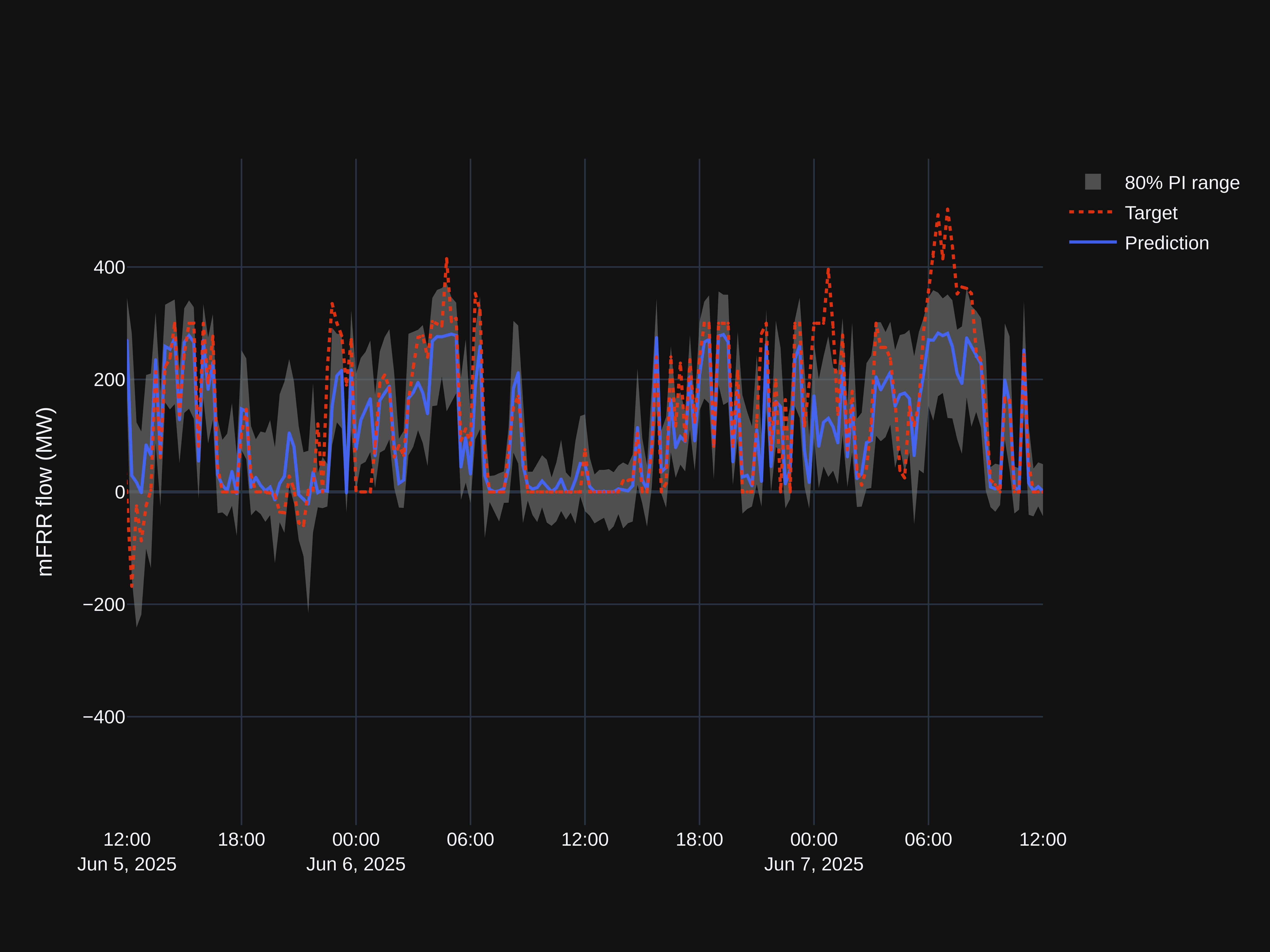
The green transition: Why the availability of power system data matters

The green transition has overwhelmed the power grid connection process for new customers. Swift and cost-effective connection relies on the expertise of power system analysts. To achieve this, Statnett believe we must enable analysts to adopt a data-driven approach akin to data scientists.

In 2019, Statnett therefore established the FRIDA program with a cross-disciplinary product team whose objective was to empower analyst by making it much easier to find and use power system data for analysis. In this post we’ll present how the team accomplished this task. The first part focuses on on the current industry challenge faced by Statnett and network operators around the world. The second part presents the tools and processes that were created to tackle it.

Overwhelming demand for grid capacity poses challenges for the power system

Statnett holds three key roles in the power system: grid owner, system operator, and transmission system network planner. We currently face challenges in:

  • Grid Connection Requests: An increasing number of requests from power producers and industrial projects, such as battery factories and data centers, demand timely responses, proper guidance for optimal project planning, and accelerated grid connection processes.
  • High Power System Utilization: During certain times of the year or when components are disconnected, the power system operates at maximum capacity. Consequently, optimizing incident management, maintenance planning, and disconnections is becoming increasingly vital.

Overall, Statnett’s decisions and services significantly impact both our customers’ value creation and the security of supply. Even minor improvements can yield considerable value.

Power system analysts require access to comprehensive amounts of data

To achieve these improvements, Statnett’s power system engineers need easy access to reliable information from various areas of the organization. They analyze vast quantities of data, including:

  • Graph model: The Common Information Model (CIM) is a comprehensive graph model that details all relevant components within the power system. It outlines connections, electrical attributes, and metadata, such as ownership. However, its complexity, consisting of millions of triplets and hundreds of data-classes, requires a level of IT knowledge that most analyst don’t have, which prevents efficient data exploration.
  • Time series: Long-term data, especially extreme values, is crucial to identify stress scenarios in the system. Given the significant influence of weather on the Norwegian power system, analysts typically require a decade’s worth of data to build confidence. For most equipment Statnett receives measurements from sensors and estimates from a network solver about every ten seconds.
  • Events: Information on faults, maintenance, and special regulations affecting system utilization is vital, along with other market data and the cost of non-delivered energy that influences bottleneck-related costs.

Traditionally, this information was only accessible through source systems or data warehouses using reports. Analysts spent 30-50% of their time locating, extracting, and ensuring data quality. To get the customers connected the analysts should spend their time finding solutions, not data.

The biggest challenge is just the sheer volume of projects. There are only so many power engineers out there who can do the sophisticated studies we need to do to ensure the system stays reliable, and everyone else is trying to hire them, too

Ken Seiler, who leads system planning at PJM Interconnection. Source: Wind and Solar Energy Projects Risk Overwhelming America’s Antiquated Electrical Grids    – The New York Times (nytimes.com)

The Power SDK makes power system data instantly available in Python

As a team we worked closely with the power system engineers to identify the areas and user stories that would be most useful to focus on. We mostly focused on creating a web app to meet their needs for finding components and studying observations related to them. This is further explained in the movie below. The movie is in Norwegian.

In the remaining part of this post, we will focus on what we did to meet the wish from our power system engineers to have the power system data instantly available in Python. The Statnett Power SDK is a Python package built on top of Statnetts data platform, to make it easier to retrive data from multiple sources and analyse this data to make better decisions.

The Power SDK was initially developed in cooperation with Cognite. Cognite Data Fusion is a part of Statnetts data platform and the primary source of information in the Power SDK. You may find the original source code here. The Power SDK has since then been further developed in Statnett. The Power SDK aims to address three common issues that made the initial user threshold too high:

  1. End users needed to connect to different databases and understand the data structure and format, which typically differed from database to database.
  2. Related data could be identified through code, but this required knowledge of graph queries and graph traversals, which most analysts lacked. For instance, adherence to the same price.
  3. The standard SDK provided by the platform used unfamiliar terms and lacked functions for typical use cases within the power analysis domain.

Below we have provided examples of how the Power SDK addresses these issues. Let’s say that an analyst needs to know the power produced in price area NO5. With the Power SDK, she may get this information through querying in terms that are familiar to how she navigates the power system mentally.

To get all substations in a price area you may write:

Python
substations = client.substations.list(bidding_area="Elspot NO5")

You may also specify the substations you want by name, voltage level, grid type and whether to include historic substations as well. You may even define areas based on the power lines entering the area. The area object will contain all the substations and power lines within the area.

From the area or list of substations you may find all connected components, such as generating units or power transformers:

Python
generating_units = substations.generating_units()

From these components you may retrieve all time series to the generators. Here I retrieve all time series of ThreePhaseActivePower related to the generators:

Python
generating_units.time_series(measurment_type="ThreePhaseActivePower")

To get events related to maintenance instead:

Python
generating_units.events(type="Driftsstans")

Once you have the time series or events, a user with basic Python skills may easily do powerful analysis. The example below shows how to find the total production in a power area over time. The area object refered to in the example could be defined by (in this example fictitious substation names):

Python
area = client.power_area(substations=['Substation1', 'Substation2']).expand_area(level=2)

or by specifying which power lines that defines the electric area.

The code below finds all relevant time series associated with the generators in the power area defined earlier, summarizes these and plots hourly values over the past year.

The analysts need guidance and support to embrace new tools

Getting busy analysts to change how they work is challenging unless you provide easy to use tools with reliable access to support. Otherwise, the barrier to trying new ways of doing things can be too significant, especially in a busy work environment. Nevertheless, we believe that the workload does not have to be large to make a change.

To provide support, we have established a common chat for users to facilitate discussions with the team and other users. Both the team and expert users can quickly provide feedback, making it easier for users to explore new approaches. Moreover, we have set up JupyterHub, enabling users without Python experience to get started faster. This also allows departments to use notebooks as lightweight dashboards, facilitating the sharing of insights.

As a result, the adoption of our Power SDK has increased dramatically, and the service has also reduced the cost and time to market for integrating other data sources for analysts. For instance, the Entsoe-py package has become popular and reduced the load on our internal data platform team.

Furthermore, helping users who encounter challenges provides us with a better understanding of their needs and pain points, facilitating the development of our products. Through our dialogue with users, we can capture the value of what we do and share our knowledge with others. For example, feedback from a user states:

Previously, I would have spent a week extracting data from the data arehouse to investigate load and flow into and through the Oslo area. Now I can create good assumptions within 1 hour.

Power System Analyst in Statnetts Regional Grid Planning department

The feedback we receive from users is useful for sharing knowledge and gaining support from management to continue our development efforts.

The analysts have used the tools to improve their methods

We are thrilled to see that analysts have a keen interest in using statistical methods to make better decisions. With our experience and expertise, we can increase the scope of data analysis and data science in Statnett, empowering analysts to generate valuable insights.

The Power SDK can also load weather data from Statnetts substations. This figure shows the relationship between the peak hourly load per day and average outdoor temperature. The figure is done by an analyst working in our long term planning department and used to assess the expected peak load in a region in Norway.

These assessments may have great economic and environmental impact as well: As the figure shows, the load is increasing at a lower rate as it gets colder. Compared to a linear trend, which was common historically, this leads to a lower expected peak demand and hence lower demand for grid capacity.

If you want more information or have ideas for cooperation, please don’t hesitate to contact us.

Writing readable mathematical code

In Statnett, we solve problems that involve a significant amount of mathematics. We need code to solve these problems, and writing readable, maintainable, testable and efficient code that computes intricate mathematical equations can be challenging. This blog post will look at one way to tackle this challenge. As a practical example, we will discuss the architectural and style choices behind the (soon to be open source) linerate Python package, which implements the conductor heat model described in CIGRE TB 601.

Dynamic line rating and CIGRE TB 601

Let’s first look briefly at the usecase we consider:  CIGRE’s Technical Brochure number 601, or CIGRE601. CIGRE601 is an essential part of our dynamic line rating work, which you can read more about in one of our previous blog posts. Here, we focus on the architectural and programming style choices we made when we developed code that implements the CIGRE 601 thermal heating model.

The mathematics of CIGRE 601 is not overly complicated, but there is a lot of it, which can make it difficult to follow if you’re not careful. At its core, CIGRE601 is a heat balance equation:

$$P_J(I) + P_s(\mathbf{w}) = P_c(T, \mathbf{w}) + P_r(T, \mathbf{w}). $$

In other words, the heating from the current ($P_J$) plus the solar heating ($P_s$) is equal to the convective cooling ($P_c$) plus the radiative (black body) cooling ($P_r$). In other words: the heating from the sun and the electricity flowing through is equal to the cooling from the wind and the radiated heat waves when the line has a constant temperature. In our case, we want to provide a current, $I$, and weather conditions, $\mathbf{w}$, and use these to solve the above equation with respect to the line temperature, $T$.

To evaluate only a single term of the above equation, we must evaluate up to another 20 other “sub-equations”. In the code, we need to keep track of all these sub-equations: what should be their input and what should be their output? We also want the implementations to be readable correct, and efficient.

Architecture

To get readable correct, and efficient code, we need to consider the software architecture. We need an architecture that strives for readability and testability without sacrificing speed (too much). How can we accomplish this?

A user-friendly frontend with a functional backend

As a basic user of a toolkit, I want to run code on the form

Python
model = Cigre601(line_parameters, weather_parameters, time)
convective_cooling = model.compute_convective_cooling(temperature)

However, we also want access to the equations themselves. While the code above is excellent for computing properties for specific lines (like the total convective cooling or ampacity rating), it could be better structured for exploring how the equations behave. To facilitate such exploration, we also want access to the sub-terms themselves.

What’s more, if we use an object-oriented approach to implement these sub-terms, then it might be appealing to store their values as properties or attributes. By doing so, we can save time on repeated computations. However, we also hide what each function depends on and provides. We want an interface that makes it clear what information we need for each computation, and if the methods implementing the equations have access to self.anything_at_all, then it is unclear what they need.

Instead, I think that a functional approach, where each mathematical equation is implemented as a pure function— a deterministic function without state — is better. Therefore, linerate has a single function for (more or less) each equation in CIGRE 601. This makes is very easy to see how the code ties together with the equations. For example, the method that computes the Joule heating is defined by

Python
def compute_joule_heating(current, resistance):
    I = current  # noqa
    R = resistance
    return I * I * R

And yes, this approach will create a minor additional computational overhead, but I found it insignificant compared to the benefits such an approach gave.

Still, I’m not saying that an object-oriented approach is only a bad thing. For linerate, we have the best of both worlds: a functional “backend” that makes it easy to explore each equation in CIGRE601 and an object-oriented “frontend” that makes it easy to compute ampacity ratings for a given power line.

Performant Python code

An essential part of mathematical code is its performance. We do not want to use native Python code for any numerical operation. Instead, we want to use the vectorisation capabilities of NumPy.

Specifically, we only use basic binary operators and NumPy universal functions (ufuncs). In the cases when we cannot use builtin ufuncs or binary operators (for example table lookups), I recommend using numba.vectorize to create your own blazing fast JIT-compiled ufuncs. By structuring the code this way, we never need to write another loop!

Say, for example, that we want to compute the line rating for all integer air temperatures between $0^\circ \text{C}$ and $6^\circ \text{C}$ and five linearly spaced wind speeds between $0 \frac{\text{m}}{\text{s}}$ and $1 \frac{\text{m}}{\text{s}}$. If we make sure that all code only uses binary operators and numpy ufuncs, then we only need to write

Python
[...]

air_temperature = np.arange(0, 7).reshape(7, 1)
wind_speed = np.linspace(0, 1, 5).reshape(1, 5)
weather = Weather(
    air_temperature=air_temperature,
    wind_speed=wind_speed
    [...]
)
model = Cigre601(weather=weather, [...])
line_rating = model.compute_steady_state_ampacity(current=2000)

The magic happens in the highlighted lines. By adding singleton axes to the array, we enable NumPy array broadcasting. Broadcasting is almost magic! Typically, when we do array computations, we need array dimensions that match up. However, singleton dimensions are “wildcards” and will match any other dimension size by repeating values in the singleton dimension until they match up. I think the best way to understand broadcasting is by computing your own multiplication table:

Python
x = np.arange(0, 5).reshape(1, 5)
y = np.arange(0, 5).reshape(5, 1)

print("x:")
print(x)
print("y:")
print(y)
print("x * y:")
print(x * y)
x:
[[0 1 2 3 4]]
y:
[[0]
 [1]
 [2]
 [3]
 [4]]
x * y:
[[ 0  0  0  0  0]
 [ 0  1  2  3  4]
 [ 0  2  4  6  8]
 [ 0  3  6  9 12]
 [ 0  4  8 12 16]]

We see that with broadcasting we can very easily compute the product of all possible combinations of entries in x and y. By only using ufuncs in our numerical code, we enable similar approaches, for example, to compute the ampacity rating for all possible combinations of weather- and line parameters.

Automatic testing of mathematical code

Okay, we got the code architecture sorted and the code super fast, so now we only need tests. Fortunately, another benefit of using pure functions for the equations is that they become straightforward to test.

Here, we will discuss two types of tests that we can make for our code: acceptance tests and property-based unit tests. The acceptance test defines a minimal set of requirements for the implementation and is provided by the standard. In CIGRE 601, we can find these under Annex E. Examples of calculation.

The more interesting part is the property-based unit tests. Property-based testing is a beautiful way to write elegant tests on the form:

given input that satisfies X, output should satisfy Y.

In Python, we use the Hypothesis library for property based testing, and I think the best way to understand it is with an example.

Consider the sorted-function. Once we sort a list, its numbers should be in ascending order, which means that lst[i] <= lst[i+1], and a test for this property could look like this:

Python
from itertools import pairwise
import hypothesis.strategies as st
from hypothesis import given


@given(lst=st.lists(st.floats()))
def test_sorted_is_ascending(lst):
    lst = sorted(lst)
    for l1, l2 in pairwise(lst):
        assert l1 <= l2

Do you think this test will pass? Click here to try it out and see for yourself!

In our case, we have mathematical equations that we want to test. And the nice thing with mathematical equations is that they have a vast amount of properties we can test! For example, the equation to compute the convective cooling, $P_c$, states that

$$ P_c = \pi \lambda_f (T_s – T_a) \text{Nu}, $$

where $\lambda_f$ is the thermal conductivity of air, $\text{Nu}$ is the Nusselt number, and $T_s$ and $T_a$ is the temperature of the conductor (surface) and air, respectively. We know that this function is linear with respect to $\lambda_f$. Moreover, if we set $T_s – T_a = \text{Nu} = 1$, then $P_c = \pi \lambda_f$, which gives us the following property-based test

Python
@given(
    thermal_conductivity_of_air=st.floats(
        min_value=0,
        max_value=1e10,
        allow_nan=False,
    )
)
def test_convective_cooling_scales_linearly_with_thermal_conductivity_of_air(
    thermal_conductivity_of_air,
):
    Nu = 1
    T_s = 1
    T_a = 0
    lambda_f = thermal_conductivity_of_air
    P_c = convective_cooling.compute_convective_cooling(T_s, T_a, Nu, lambda_f)
    
    assert P_c == np.pi * approx(lambda_f)

Here, we let Hypothesis select arbitrary values for $\lambda_f$, and only test whether whether $P_c = \pi \ \lambda_f$ when $\text{Nu} = T_s – T_a = 1$. If we didn’t use Hypothesis, we would either have to hard-code the test cases (e.g. with pytest.mark.parametrize) or iterate over random values for $\lambda_f$, which would make it less obvious what the code actually tests.

Style considerations

Selecting good variable names

One of the first style considerations we encounter when implementing mathematical equations with code is what we should name our variables. Do we use mathematical symbols or semantic names for the variable names?

Recall the equation for the convective cooling:

$$ P_c = \pi \lambda_f (T_s – T_a) \text{Nu}. $$

With Python, we could write the following equivalent function:

Python
def compute_convective_cooling(
    lambda_f: float,
    T_s: float,
    T_a: float,
    Nu: float,
) -> float:
    r"""Compute the convective cooling of the conductor.

    Equation (17) on page 24 of :cite:p:`cigre601`.
    """
    return pi * lambda_f * (T_s - T_a) * Nu

However, while this makes it easy to see how the mathematics works, it could be more user-friendly. For example, do you remember what lambda_f represents?

We could, of course, switch it around and use argument names with semantic meaning:

Python
def compute_convective_cooling(
    thermal_conductivity_of_air: float,
    surface_temperature: float,
    air_temperature: float,
    nusselt_number: float,
) -> float:
    r"""Compute the convective cooling of the conductor.

    Equation (17) on page 24 of :cite:p:`cigre601`.
    """
    return pi * thermal_conductivity_of_air * (surface_temperature - air_temperature) * nusselt_number

but then it becomes challenging to connect the code and the equations.

To get code where the variables both have semantic meaning, and the equations are easy to follow, we can combine these two approaches:

Python
def compute_convective_cooling(
    thermal_conductivity_of_air: float,
    surface_temperature: float,
    air_temperature: float,
    nusselt_number: float,
) -> float:
    r"""Compute the convective cooling of the conductor.

    Equation (17) on page 24 of :cite:p:`cigre601`.
    """
    lambda_f = thermal_conductivity_of_air
    T_s = surface_temperature
    T_a = air_temperature
    Nu = nusselt_number
    return pi * lambda_f * (T_s - T_a) * Nu

This way, the API clarifies what we need to know to compute the convective cooling, while it is also easy to compare the code with the reference equations.

Selecting good function names

One of my main pet peeves when I deal with mathematical code is function names. All functions (unless you have a very good reason) should have a verb in their name. After all, a function does do something, so why not explicitly state what it does?

In mathematical code, naming functions with verbs is even more critical. Take, for example, the convective_cooling function we defined above. The function is very readable. We see what the inputs are, what it computes and how. Still, if we want to use this function to compute some convective cooling, we should also give that variable a good name. Any suggestions for a good name? I would probably want to go with convective_cooling. But wait, that’s the name of the function, so we might end up writing

Python
convective_cooling = convective_cooling([...])

This is not ideal.

What is the solution to the naming problem? Simply add a verb to the function name. For example, “compute”:

Python
def compute_convective_cooling(
    thermal_conductivity_of_air,
    surface_temperature,
    air_temperature,
    nusselt_number,
):
    r"""Compute the convective cooling of the conductor.

    Equation (17) on page 24 of :cite:p:`cigre601`.
    """
    lambda_f = thermal_conductivity_of_air
    T_s = surface_temperature
    T_a = air_temperature
    Nu = nusselt_number
    
    return lambda * (T_s - T_a) * Nu


convective_cooling = compute_convective_cooling(
    thermal_conductivity_of_air=thermal_conductivity_of_air,
    surface_temperature=surface_temperature,
    air_temperature=air_temperature,
    nusselt_number=nusselt_number,
)

Sure, the function names get longer, but the code also becomes much more pleasant to read!

Using typing.annotated to provide units

A handy new Python feature (3.9) is annotated types. Annotated types allow us to provide extra information to our type hints. This is very useful for physical equations, where we can use the annotations to represent units. In linerate, we do this in the units.py-file

Python
from typing import Union

try:
    from typing import Annotated
except ImportError:  # Python version <3.9
    from typing_extensions import Annotated

import numpy as np
import numpy.typing as npt

FloatOrFloatArray = Union[float, np.float64, npt.NDArray[np.float64]]

OhmPerMeter = Annotated[FloatOrFloatArray, "Ω/m"]
Ampere = Annotated[FloatOrFloatArray, "A"]
Radian = Annotated[FloatOrFloatArray, "rad"]

We use these annotations in the functions that implement the mathematical equations:

def compute_joule_heating(current: Ampere, resistance: OhmPerMeter) -> WattPerMeter:
    I = current  # noqa
    R = resistance
    return I * I * R

Using annotations like this makes it extraordinarily easy to know what units we use in the different functions. But unfortunately, the units are not type-checked, so we can still write the wrong units by accident. I’m hopeful that a package like Pint can provide static checking of units in the future, but that is not possible (at least for now).

Extensive use of documentation strings

I believe docstrings are particularly important when we implement mathematical equations. A bare minimum is listing the source of the equations (e.g. Equation (17) on page 24 of CIGRE TB 601.). Even better, if you’re using Sphinx for the documentation, you can include the sphinxcontrib.bibtex plugin, which enables you to link the documentation against a BibTeX database (e.g. Equation (17) on page 24 of :cite:p:`cigre601`.).

After listing which equation(s) each function represents, we may want also to describe the notation. I like using the function arguments and returns field of the docstring for this, preferably formatted with LaTeX and using either the NumPy docstring style or the Google docstring style. A nice benefit we get by including type hints is that Sphinx can automatically parse these to provide the types in the docstring, also. To enable this, set

Python
autodoc_typehints = "description"
autodoc_typehints_description_target = "documented"

in the Sphinx conf.py file. Unfortunately, I have yet to figure out how to get it to include the return types properly, but at least we don’t need to worry about the input types.

A final and somewhat optional step is to also include information about the quantities in the docstring so that the user does not need to look at the references. If we combine all these steps, we get a docstring kind of like the one below

Python
def compute_convective_cooling(
    surface_temperature: Celsius,
    air_temperature: Celsius,
    nusselt_number: Unitless,
    thermal_conductivity_of_air: WattPerMeterPerKelvin,
) -> WattPerMeter:
    r"""Compute the convective cooling of the conductor.

    Equation (17) on page 24 of :cite:p:`cigre601`, given by
    
    .. math::
    
        P_c = \lambda_f \ Nu \ (T_a - T_s).

    Parameters
    ----------
    surface_temperature:
        :math:`T_s~\left[^\circ\text{C}\right]`. The conductor surface temperature.
    air_temperature:
        :math:`T_a~\left[^\circ\text{C}\right]`. The ambient air temperature.
    nusselt_number:
        :math:`Nu`. The nusselt number.
    thermal_conductivity_of_air:
        :math:`\lambda_f~\left[\text{W}~\text{m}^{-1}~\text{K}^{-1}\right]`. The thermal
        conductivity of air at the given temperature.

    Returns
    -------
    Union[float, float64, ndarray[Any, dtype[float64]]]
        :math:`P_c~\left[\text{W}~\text{m}^{-1}\right]`. The convective cooling of the conductor.
        Either due to wind, or passive convection, whichever is largest.
    """

Closing notes

There is no single solution to writing maintainable and readable mathematical code. This blog post demonstrates the choices behind linerate, but I am sure there are ways to improve these decisions. My main pain point is units, and for a future project, I hope to check if Pint might be part of a solution to ensuring consistent type usage. Moreover, I would test the code more thoroughly if given infinite time. For example, instead of checking that a function is linear by fixing all parameters but one, we could numerically differentiate it and check that the derivative is constant almost everywhere. If you have any ideas for writing maintainable and readable mathematical code, please share them in the comments below!

Cimsparql: Loading power system data into pandas dataframes in Python

In 2019, we started working on a model that should be able to handle intra-zonal constraints in the upcoming balancing market. That methodology has been presented in a previous post in January 2022. In this post, we will focus on an open source Python library called cimsparql that we have developed to support this model. For the model to be able to perform any analysis, it needs data that describe the state of the power system. At Statnett, these data are available as CIM (Common Information Model) profiles. The data is made available through a triple store (GraphDB/Blazegraph/rdf4j), using a resource description framework which is a standard model for data interchange.

The information about the power system available in these CIM profiles can be used for different purposes, and what information should be extracted depends on the requirement of your model. In the previously presented post, a DC optimal power flow model is used. Thus we need data on generation, demand and transmission lines. The purpose of the cimsparql package is to extract this information from the triple store, through a set of predefined sparql queries, and loading them into Python as pandas dataframes. Cimsparql will also make sure that columns in the dataframes have correct types, either string, float or integer, as defined by the CIM standard.

Cimsparql uses the SPARQLWrapper library to remotely execute sparql queries, and extends it with extra functionality, assuming the data conform to the CIM standard. Even though the package is an important part of the balancing market model, it is open source available from github and can be installed using pip.

~/pip install cimsparql

Once the library is installed, it must be configured to query a triple store using the ServiceConfig class in cimsparql.graphdb. The example below assumes you have a graphdb server with a CIM model in a repository called “micro_t1_nl”. This test case, available at the cimsparql repository on github, is used to test the development of the predefined queries.

  >>> service_cfg = ServiceConfig(repo="micro_t1_nl")
  >>> model = get_cim_model(service_cfg)

If you need to provide other configurations such as server, username and password, this can be done with the same ServiceConfig class.

Once the model is configured, the data can be loaded into a pandas dataframe using the predefined queries. In the example below, topological node information is extracted from the triple store.

>>> bus = model.bus_data()
>>> print(bus.to_string())
                                           busname      un
node                                                      
795a117d-7caf-4fc2-a8d9-dc8f4cf2344a  NL_Busbar__4  220.00
6bdc33de-d027-49b7-b98f-3b3d87716615   N1230822413   15.75
81b0e447-181e-4aec-8921-f1dd7813bebc   N1230992195  400.00
afddd60d-f7e6-419a-a5c2-be28d29beaf9   NL-Busbar_2  220.00
97d7d14a-7294-458f-a8d7-024700a08717    NL_TR_BUS2   15.75

Here the values in the nominal voltage column has been converted to float values as defined by the CIM standard, while node and bus names are strings.

All the predefined queries can be executed using the cimsparql.model.CimModel class. Examples are the already shown bus_data as well as loads, synchronous_machines, ac_lines and coordinates. The latter extracts coordinates of all equipment in the model from the CIM Geographical Location profile. Cimsparql orders the rows in the dataframe such that it is straightforward to use with plotly’s map functionality. The example below was made in a Jupyter notebook.

df = model.coordinates()
lines = df.query("rdf_type == 'http://iec.ch/TC57/2013/CIM-schema-cim16#ACLineSegment'")
stations = df.query("rdf_type == 'http://iec.ch/TC57/2013/CIM-schema-cim16#Substation'")
center_x, center_y = df["x"].mean(), df["y"].mean()

fig = px.line_mapbox(lines, lon="x", lat="y", color="mrid", height=1000)
fig2 = px.scatter_mapbox(stations, lon="x", lat="y", color="mrid", size=[1]*len(stations))
fig.update_geos(countrycolor="black", showcountries=True, showlakes=True, showrivers=True, fitbounds="locations")
fig.update_layout(mapbox_style="stamen-terrain")

all_fig = go.Figure(data=fig.data + fig2.data, layout = fig.layout)
all_fig.show()
AC line segments and substations included in the model

The main goal of cimsparql is to read data for the purpose of running power flow analysis using sparql queries to read data from triple store into pandas dataframes in Python. Currently the package is used internally at Statnett, where we also have some data which is yet not covered by the CIM standard. Thus some of the queries contains a namespace which will probably only be used by Statnett. However, this should not pose any problem for the use of this package elsewhere, as these namespaces or columns have been made optional. So any query towards a data set that does not contain these, will just produce a column for the given namespace with NaN values.

The package can also be uses in cases where the predefined queries does not produce data for a specific purpose. In this case, the user can provide their own queries as a string argument to the get_table_and_convert method. The example below list out the numbers of ac line segments for each voltage level in your data.

>>> query='''
PREFIX cim: <http://iec.ch/TC57/2013/CIM-schema-cim16#>
PREFIX rdf: <http://www.w3.org/1999/02/22-rdf-syntax-ns#>
select ?un (count(?mrid) as ?n) where { 
?mrid rdf:type cim:ACLineSegment;
   cim:ConductingEquipment.BaseVoltage/cim:BaseVoltage.nominalVoltage ?un.
} group by ?un'''
>>> df = model.get_table_and_convert(query)

So to summarize, the main contribution of cimsparl is a set of predefined queries for the purpose of running power flow simulations and type conversion of data that follows the CIM standard.

Julia: A powerful alternative to Python

Almost three years ago, I started on my journey towards an industrial PhD in reinforcement learning applied to power systems. At around that time, I had used Python daily for 6-7 years. But one day during the autumn of 2018, Thomas, the founder of our Data Science team, threw out a new idea to me, like he used to do at the time: "Have you ever tried Julia? You really should! Some guys at MIT were tired of the slowness and problems with Python so they decided to create a new language. And there’s a module for power systems too, the PowerModels.jl." So there it started for me. And at the start my PhD project I thought it was a good opportunity for me to learn a new programming language from scratch along the way.

Getting started with Julia

If you don’t have Julia installed already, I suggest you install it now so you can follow along through the rest of this post. If you’re on Linux, the easiest way to get the installation of Julia up and running is to use juliaup:

curl -fsSL https://install.julialang.org | sh

or have a look at the Julia homepage.

Once you’re up and running, the easiest way to install a package when you’re in
a Julia session is to just start using it by typing using <package name>, as
for example in


julia> using Plots
 │ Package Plots not found, but a package named Plots is available from a registry. 
 │ Install package?
 │   (@v1.8) pkg> add Plots 
 └ (y/n/o) [y]: 

Julia seeks to solve the two-language problem

Julia is an open-source, high-level, dynamically-typed language. It was started back in 2009 by a group of people at MIT: Stefan Karpinski, Jeff Bezanson, Viral B. Shah and Alan Edelmann. The first version was released in 2012. In their blogpost from february 2012, the authors stated they wanted a programming language "… [with] the speed of C… as usable for general programming as Python…, [and] as easy for statistics as Matlab". Following this, Julia seeks to solve the two-language problem. If you want a language that is dynamic, flexible and easy to prototype in, you usually have to sacrifice speed, as in Python and R. On the other hand, if you want performance-critical code you have to resort to fast, static and compiled languages such as C and C++.

The way Julia solves this is by having a native, feature-rich REPL (Read-Eval-Print Loop) and by having JIT (just in time)-compilation together with a flexible, parametric type system along with multiple dispatch. More on this later!

The Julia REPL is your best friend

When prototyping in Julia, the natural starting point is the Julia REPL, which in many ways behaves pleasantly like the iPython interface but also with so much more. The Julia REPL has four main modes (together with full history search):

  • The Julia code prompt
  • Help mode
  • Package manager
  • Shell mode

1) The standard Julia code prompt

This mode is invoked at startup and is the mode where you do all your prototyping. For example, illustrating 3 different ways to write a function:

add_one_line(x) = x + 1 # one-line
add_one_anon = x -> x + 1 # anonymous function
function add_one_full(x)
    return x + 1
end

2) The help mode

This is invoked by typing ? and give you quick access to the docstring of a function. So if we are in Julia prompt mode and type

"""
    myadd(x,y)

Add x and y.
"""
function myadd(x,y)
    return x + y
end

we can activate the help mode by typing ? and then type the function name:

help?> myadd
search: myadd

  myadd(x,y)

  Add x and y.

3) The package manager

Apart from the speed, this is perhaps my favourite feature of the Julia language. In Python, there are number of different environment and package managers, like "pip", "pipenv", "virtualenv" and "poetry". Choosing between them and understanding how they work together can be confusing and time-consuming. In Julia, the package manager is built into the language and it just works. The package manager is invoked by typing ] and you leave it by typing backspace. In an empty directory you can create a new environment like this:

(@v1.7) pkg> activate .
  Activating new project at `~/JuliaProjects/sandbox/blog`

(blog) pkg> add UnicodePlots
    Updating registry at `~/.julia/registries/General.toml`
   Resolving package versions...
    Updating `~/JuliaProjects/sandbox/blog/Project.toml`
  [b8865327] + UnicodePlots v3.1.0
    Updating `~/JuliaProjects/sandbox/blog/Manifest.toml`
  ...

(blog) pkg> 
julia> 

This can also be done programatically in the Julia REPL like this:

julia> using Pkg; Pkg.add("UnicodePlots")
    Updating registry at `~/.julia/registries/General.toml`
   Resolving package versions...
    Updating `~/.julia/environments/v1.7/Project.toml`
  [b8865327] + UnicodePlots v3.1.0
    Updating `~/.julia/environments/v1.7/Manifest.toml`
 ...

An environment is defined by two .toml-files. The Project.toml contains the packages you want in the environment together with version restrictions. The Project.toml is the file to commit to github. The file Manifest.toml is the detailed machine-generated file which contains all the information necessary to exactly reproduce a specific environment. Both files are constructed when you instantiate an environment and updated automatically when you add new packages.

4) The shell mode

By typing ; in the REPL you get instant access to a shell that behaves like a bash shell, which in many occasions could be really handy. But in practice I usually just open a new terminal with my regular bash shell.

Julia is not object-oriented – it relies on multiple dispatch

On the surface, the Julia syntax doesn’t differ too much from Python, the main differences being 1-based indexing and that functions and control structures in Julia are always closed by the end keyword. And as in Python, you don’t need to annotate the type of the variable. In this context, an important part of Julia, is the type inference. This means that the types are inferred from the actual variable values. For example,

julia> a = 1; typeof(a)
Int64

julia> a = 1.0; typeof(a)
Float64

julia> a = "Hello, word"; typeof(a)
String

julia> a = 1 + 1.0f0; typeof(a)
Float32

One main difference from Python is that Julia is not objected-oriented, so there are no classes and inheritance. Instead, Julia has a very flexible type hiearchy, with C-like structs as the main building block. This means that functions don’t belong to certain types or objects as they do in Python. Instead, Julia has polymorphism where functions can have the same name but which function to be used at runtime, or dispatched, depends on the types of the arguments of the function call. I write arguments in plural, because Julia has so called multiple dispatch, meaning that the language considers the types of all the arguments when choosing which function to execute. This is a remarkable feature. Let me show an example:

struct MyNumber
    x::Float64
end

f(x) = "I am the fallback for one argument" 
f(x::Integer) = "I'm dispatched on integers"
f(x::Float64) = "I'm dispatched on floats"
f(x, y) = "Fallback for two arguments"
f(x::Int, y::Float64) = "First is Integer, second argument is Float64"
f(x::MyNumber) = "Hello, mynumber!"

mynumber = MyNumber(1.0)

f("Hello, world!")  # I am the fallback for one argument
f(1)  # I'm dispatched on integers
f(1.0)  # I'm dispatched on floats
f("Hello", 1)  # Fallback for two arguments
f(1, 2.0)  # First is Integer, second argument is Float64
f(mynumber)  # "Hello, mynumber!"

Julia is compiled just-in-time

This brings me to the second main difference: Julia is compiled. The compilation is done at runtime by a so-called JIT (just-in-time) compiler. JIT-compilation is also found in for example the Numba library in Python. In the example above, we have six different versions of the function called f. These versions are called methods in Julia. We can examine what methods of the function f above are actually defined by calling the methods function on f:

julia> methods(f)
# 6 methods for generic function "f":
[1] f(x::Int64, y::Float64) in Main at REPL[6]:1
[2] f(x::Integer) in Main at REPL[3]:1
[3] f(x::Real) in Main at REPL[4]:1
[4] f(x::MyNumber) in Main at REPL[7]:1
[5] f(x) in Main at REPL[2]:1
[6] f(x, y) in Main at REPL[5]:1

So at runtime, when the program is about to execute a specific function call, the compiler checks the types of all the actual input arguments of the function. If it has been called and compiled before with this combination of argument types, it uses a cached version, which of course is very fast. If not, a new version based on all the argument types of the current call is compiled and stored. This means we only need to compile functions actually used in the code.

Julia is fast because of code specialization

In principle, Julia code can get the speed of C for any user-defined type. This is in contrast to for example numpy in Python, where the speedups only apply to a limited collection of predefined datatypes. Compared to native Python, the speedup naturally varies a lot depending on the task, but figures of 2-10 times faster are not unheard of.

Even though modern data science tools in Python like Numpy and Tensorflow are wrappers around C/C++ and with that bring speed to the table, it is still useful to understand why pure Python is slow.

Coming from Python to Julia, the biggest change for me was to become more aware of the types of the variables and objects you are actually doing things with. "Is this an array of 64-bit floats?" "What are the types of the class members?" Working in pure Python, none of these questions seemed relevant because in Python a variable could bascially be of any type and things just still work.

So for example, when you want to sum an array of values in Python, each and every time you add two values the langauge needs to check the type of the values and at runtime find the right +-function to use in the summation and store the resulting value together with its type. There is no way to inform the language that all the values of an array are the same type, for example 64-bit precision floats.

How slow this is can actually be illustrated in Julia, where the type Any is the mother of all types and of which all other types is a subtype. The Julia type Any is equivalent to the the Python generic type. By using the Julia package BenchmarkTools we can compute statistics on the time spent on summing 10^7 random numbers in an array.

julia> using BenchmarkTools
julia> N = 10^7
julia> arr_any = Any[rand() for i in 1:N];
julia> arr_float64 = Float64[rand() for i in 1:N];
julia> @benchmark sum($arr_any)
BenchmarkTools.Trial: 31 samples with 1 evaluation.
 Range (min … max):  135.170 ms … 169.061 ms  ┊ GC (min … max):  0.00%16.89%
 Time  (median):     165.452 ms               ┊ GC (median):    16.91%
 Time  (mean ± σ):   163.840 ms ±   7.513 ms  ┊ GC (mean ± σ):  16.03% ±  4.23%

                                                       ▂█ ▄      
  ▄▁▁▄▁▁▁▁▁▁▁▁▁▁▁▁▁▁▁▁▁▁▁▁▁▁▁▁▁▁▁▁▁▁▁▁▁▁▁▁▁▁▁▁▁▁▁▁▁▁▆▆▄████▆▄▄▄ ▁
  135 ms           Histogram: frequency by time          169 ms <

 Memory estimate: 152.59 MiB, allocs estimate: 9999999.

julia> @benchmark sum($arr_float64)
BenchmarkTools.Trial: 1193 samples with 1 evaluation.
 Range (min … max):  4.047 ms …  4.706 ms  ┊ GC (min … max): 0.00%0.00%
 Time  (median):     4.165 ms              ┊ GC (median):    0.00%
 Time  (mean ± σ):   4.181 ms ± 78.071 μs  ┊ GC (mean ± σ):  0.00% ± 0.00%

         ▂▁▄▆██▅▆▇▂▃▅▅▃▄▂                                     
  ▂▂▂▃▃▆▅█████████████████▇█▇▆▅▆▄▄▄▇▃▅▃▃▄▄▃▃▃▂▃▂▁▂▁▂▁▂▂▁▁▁▁▁ ▄
  4.05 ms        Histogram: frequency by time        4.42 ms <

 Memory estimate: 0 bytes, allocs estimate: 0.

As we can see, the compiler does its job and the median execution time is about 40 times slower with the generic type where the compiler cannot specialize on the type of the argument.

SINTEF and viralinstruction have written two very helpful blogposts that elaborate on how to get performant Julia code. In the Julia manual, there is a dedicated section on performance tips. I also highly recommend Steven Johson’s MIT lecture on Julia.

Julia has a growing ecosystem

The ecosystem of Python is impressive and mature. And the current era of Data Science has more or less evolved hand in hand with Python and its machine learning libraries such as SciPy and Tensorflow. Python was first released in 1991, more than twenty years before Julia. And as of september 2022, there are 400 000 projects in PyPi. In comparison, Julia has at the same time about 8 000 registered packages. In fact, already in 2017, Stefan Karpinski stated that:

Even NumPy itself was a bit rough back then. It’s entirely possible that if the SciPy ecosystem had been as well developed in 2009 as it is today, we never would have started Julia.

But the number of users and packages in Julia is growing, and I’ve definitely found what I need. To name a few I’ve used, there’s the Plots.jl and Makie.jl for plotting. There’s the Pandas equivalent DataFrames.jl for dataframes. There’s Flux.jl for machine learning. There’s ReinforcementLearning.jl for reinforcement learning, obviously. And there’s the PowerModels.jl for dealing with power systems.

Even though not all packages are as far developed as in Python, this has not been a major problem for me. And there are some benefits too of entering a package in its early phase. Your issues and requests have a better chance of being taken care of and it’s quite possible you are able to contribute to the project yourself, either with code or documentation. The two packages I’ve been deepest involved with, ReinforcementLearning.jl and GraphNeuralNetworks.jl, both have very friendly and helpful core developers.

A nice little Julia package: UnicodePlots.jl

I have to mention this neat little package in Julia, UnicodePlots.jl, which allows you to do simple plotting in the command line. For example,

using UnicodePlots

lineplot([cos, sin], 0:0.01:2pi)
barplot(["Oslo", "Stavanger", "Bergen", "Trondheim"],
        [2.244, 8.406, 4.92, 0.1],
        title = "Population")

which in my terminal renders as

How can Julia be used in power systems research?

My PhD project is about how to use reinforcement learning to handle failures in the power system. This involves a lot of load flow calculations. This is super easy in PowerModels.jl:

using PowerModels
# Casefile "case.14m" downloaded from https://egriddata.org/sites/default/files/case14.m

julia> results = compute_dc_pf("case14.m")
...
Dict{String, Any} with 5 entries:
  "optimizer"          => "\\"
  "termination_status" => true
  "objective"          => 0.0
  "solution"           => Dict{String, Any}("bus"=>Dict{String, Any}("4"=>Dict("va"=>-0.200698), "1"=>Dict("va"=>-0.0), "12"=>Dic…
  "solve_time"         => 0.000584841

Perhaps even more useful is to do an optimal power flow using the Ipopt.jl optimizer:

julia> using PowerModels
julia> using Ipopt

julia> solve_dc_opf("case14.m", Ipopt.Optimizer)

...

Number of nonzeros in equality constraint Jacobian...:      106
Number of nonzeros in inequality constraint Jacobian.:       80
Number of nonzeros in Lagrangian Hessian.............:        5

Total number of variables............................:       39
                     variables with only lower bounds:        0
                variables with lower and upper bounds:        5
                     variables with only upper bounds:        0
Total number of equality constraints.................:       35
Total number of inequality constraints...............:       40
        inequality constraints with only lower bounds:       20
   inequality constraints with lower and upper bounds:        0
        inequality constraints with only upper bounds:       20

iter    objective    inf_pr   inf_du lg(mu)  ||d||  lg(rg) alpha_du alpha_pr  ls
   0  1.6032287e+02 9.32e-01 1.89e+01  -1.0 0.00e+00    -  0.00e+00 0.00e+00   0
   1  8.6948059e+03 1.46e-16 6.86e+01  -1.0 7.93e-01    -  1.41e-02 1.00e+00h  1
   2  7.6460391e+03 6.66e-16 2.59e+00  -1.0 1.43e+00    -  5.95e-01 9.60e-01f  1
   3  7.6605209e+03 5.48e-16 3.39e+00  -1.0 1.48e-01    -  9.76e-01 5.00e-01f  2
   4  7.6544392e+03 6.66e-16 1.00e-06  -1.0 3.40e-02    -  1.00e+00 1.00e+00f  1
   5  7.6457228e+03 5.76e-16 2.83e-08  -2.5 5.25e-02    -  1.00e+00 1.00e+00f  1
   6  7.6432829e+03 4.44e-16 2.83e-08  -2.5 1.85e-02    -  1.00e+00 1.00e+00f  1
   7  7.6426423e+03 3.89e-16 1.50e-09  -3.8 5.43e-03    -  1.00e+00 1.00e+00f  1
   8  7.6425922e+03 6.66e-16 1.84e-11  -5.7 4.35e-04    -  1.00e+00 1.00e+00f  1
   9  7.6425918e+03 3.37e-16 2.51e-14  -8.6 3.75e-06    -  1.00e+00 1.00e+00f  1

Number of Iterations....: 9

                                   (scaled)                 (unscaled)
Objective...............:   1.9106479435807935e+02    7.6425917743231739e+03
Dual infeasibility......:   2.5059035640133008e-14    1.0023614256053203e-12
Constraint violation....:   3.3653635433950058e-16    3.3653635433950058e-16
Variable bound violation:   8.9305948524944555e-09    8.9305948524944555e-09
Complementarity.........:   2.6421734022358593e-09    1.0568693608943436e-07
Overall NLP error.......:   2.6421734022358593e-09    1.0568693608943436e-07


Number of objective function evaluations             = 11
Number of objective gradient evaluations             = 10
Number of equality constraint evaluations            = 11
Number of inequality constraint evaluations          = 11
Number of equality constraint Jacobian evaluations   = 1
Number of inequality constraint Jacobian evaluations = 1
Number of Lagrangian Hessian evaluations             = 1
Total seconds in IPOPT                               = 0.005

EXIT: Optimal Solution Found.
Dict{String, Any} with 8 entries:
  "solve_time"         => 0.00622511
  "optimizer"          => "Ipopt"
  "termination_status" => LOCALLY_SOLVED
  "dual_status"        => FEASIBLE_POINT
  "primal_status"      => FEASIBLE_POINT
  "objective"          => 7642.59
  "solution"           => Dict{String, Any}("baseMVA"=>100, "branch"=>Dict{String, Any}("4"=>Dict{String, Any}("qf"=>NaN, "qt"=>N…
  "objective_lb"       => -Inf

Deep learning in Julia? Use Flux!

Flux.jl is the go-to library for deep learning in Julia. It is the Tensorflow and Pytorch equivalent.

Let’s do a simple example on training a linear regression model with intercept at 1.5 and slope 2.0. We first start by importing the necessary library and defining our data:

julia> using Flux
julia> x = rand(Float32, 1, 100)
#1×100 Matrix{Float32}:
# 0.971723  0.279388  0.718561  0.580433  0.319538  0.571858  0.808591  0.967042  0.511453  0.824858  0.0246731  0.924845  0.804781  0.0334803  0.864933  0.561797  0.459436  0.134477  0.397105  …  0.885082  0.444496  0.891089  0.452616  0.0905207  0.258379  0.736683  0.28399  0.624088  0.604748  0.275982  0.696864  0.735082  0.959392  0.580974  0.75722  0.763027  0.0576547

julia> intercept = 1.5
julia> slope = 2.0
julia> linear_noise(x, ϵ=0.1) = intercept + slope*x + randn()*ϵ
# linear_noise (generic function with 2 methods)

julia> y = linear_noise.(x) .|> Float32
#1×100 Matrix{Float32}:
# 3.25849  2.26917  2.8143  2.85554  2.12951  2.77449  3.19595  3.5636  2.56589  3.22538  1.59178  3.22211  3.02087  1.59712  3.15416  2.68378  2.3113  1.82769  2.43546  3.04249  2.02023  3.20036  …  1.91827  1.88766  3.24948  2.37444  3.17674  2.45275  1.57015  2.00188  2.83694  2.09291  2.79805  2.75575  2.06506  2.73183  2.99427  3.38747  2.55995  3.17439  3.12668  1.64066

The piping operator |> is very handy in Julia, the same is the broadcasting done by the .-operator. See the manual for more informations about these.

So now we have linear data with some noise added. Let’s also define a very simple neural network, with 1 layer and only one node. As we can see, there are two parameters in this model:

julia> model = Dense(1,1)
# Dense(1 => 1)       # 2 parameters

We can get the parameters of the model, a.k.a. the weights and the biases, by

julia> ps = Flux.params(model)
# Params([Float32[0.819971;;], Float32[0.0]])

We also define a loss function by

julia> loss(input, output) = Flux.Losses.mse(model(input), output)
# loss (generic function with 1 method)

julia> loss(x, y)
# 11.150247f0

So with random weight and bias, the loss is initially quite large. Let’s implement a simple gradient descent, loop over the data and train on the cpu (which is the default):

julia> epochs = 10_000

julia> opt = Flux.Descent()  # 0.1 is the default step size
# Descent(0.1)

julia> for epoch in 1:epochs
           ps = Flux.params(model)
           Flux.train!(loss, ps, [(x,y)], opt)
       end

julia> loss(x,y)
# 0.009441698f0

julia> Flux.params(model)
# Params([Float32[1.9716092;;], Float32[1.5128096]])

Finally let’s plot the results using the standard Plots.jl library using the GR backend:

julia> using LaTeXStrings
julia> using Plots

julia> gr() # to activate the GR backend (not necessary as it is the default)
# Plots.GRBackend()

julia> p = scatter(x[1,:],y[1,:], label="observations", legend=:topleft, xlabel=L"x", ylabel=L"y")
julia> plot!(p, x[1,:], model(x)[1,:], label="model")

In the last function call, we see an example of a Julia convention: Any function that changes the argument in place has an "!" at the end of the identifier.

What’s not to like?

Time to first plot

The first time a Julia method is called it is compiled and this obviously prolongs the execution time. Sometimes this can lead to some delays (and frustration) when you’re typing interactively. Every time you close the Julia session and start a new one, you have to go throuh the compilations again. This manifests itself also in the so-called Time To First Plot (TTFP). Although this has been improved in almost every release of Julia, you still have two wait some long seconds. For example, these lines of code takes about 8s on my terminal from a fresh Julia session:

using Plots
x = range(0, 2pi, length=100)
plot(x, sin.(x))

Of course, the second time these lines are run from the same session it runs instantaneously.

In Python, the equivalent code took much less than 1s:

import matplotlib.pyplot as plt
import numpy as np

x = np.linspace(0, 2*np.pi, num=100, endpoint=True)
plt.plot(x, np.sin(x))
plt.show()

Debugging

The Julia debugger is also one part of Julia that has not brought forth the best of my feelings. Although it also has improved recently, to be frank I don’t use it much. In Python I used to step through the code in for example the Pycharm IDE. This gave much insight. In Julia, I code much more interactively through the REPL. I also implement shorter functions that are more testable and in a functional programming style. In addition, I use tools like Infiltrator.jl. After a year of coding like this, I hardly miss a debugger.

Closing remarks

To me, learning Julia has been a very positive experience. Julia is fast, fun to read and write, and it is applicable to a wide range of computational problems. But maybe more importantly, by learning a new language I have learned a lot on how computers and programming languages work together. And I have learned that there are alternatives to the Pythonic way. So if in doubt: Give Julia a try!

Is bid filtering effective against network congestion?

Earlier this year, I wrote an introduction to the bid filtering problem, and explained how my team at Statnett are trying to solve it. The system we’ve built at Statnett combines data from various sources in its attempt to make the right call. But how well is it doing its job? Or, more precisely, what is the effect on network congestion of applying our bid filtering system in its current form?

Kyoto. Photo: Belle Co

Without calling it a definitive answer, a paper I wrote for the CIGRE Symposium contains research results that provide new insight. The symposium was in Kyoto, but a diverse list of reasons (including a strict midwife) forced me to leave the cherry blossom to my imagination and test my charming Japanese phrases from a meeting room in Trondheim.

A quick recap

European countries are moving toward a new, more integrated way of balancing their power systems. In a country with highly distributed electricity generation, we want to automatically identify power reserves that should not be used in a given situation due to their location in the grid. If you would like to learn the details about the approach, you are likely to enjoy reading the paper. Here is the micro-version:

To identify bids in problematic locations, we need a detailed network model, we try to predict the future situation in the power grid, and then we apply a nodal market model which gives us the optimal plan for balancing activations for a specific situation. But since we don’t really know how much is going to flow into or out of the country, we optimize many times with different assumptions on cross-border flows. Each of the exchange scenarios tells its own story about which bids should -and shouldn’t- be activated. The scenarios don’t always agree, but in the aggregate they let us form a consensus result, determining which bids will be made unavailable for selection in the balancing market.

An unfair competition

Today, human operators at Statnett select power reserves for activation when necessary to balance the system, always mindful of their locations in the grid and potential bottlenecks. Their decisions on which balancing bids to activate – and not activate – often build years of operational experience and an abundance of real-time data.

Before discussing whether our machine can beat the human operators, it’s important to keep in mind that the bid filtering system will take part in a different context: the new balancing market, where everyday balancing will take place without the involvement of human operators. This will change the rules of the balancing game completely. While human operators constantly make a flow of integrated last-minute decisions, the new automatic processes are distinct in their separation of concerns and must often act much earlier to respect strict timelines.

Setting up simulations

The quantitative results in our paper come from simulating one day in the Norwegian power grid, using our detailed, custom-built Python model together with recorded data. The balancing actions -and the way they are selected- are different between the simulations.

The first simulation is Historical operation. Here, we simply replay the historical balancing decisions of the human operators.

The second simulation is Bid filtering. Here, we replace the historical human decisions with balancing actions selected by a zonal market mechanism that doesn’t see the internal network constraints or respect the laws of physics. The balancing decisions will often be different from the human ones in order to save some money. But before the market selects any bids, some of them are removed from the list by our bid filtering machine in order to prevent network congestion. We try not to cheat, the bid filtering takes place using data and forecasts available 30 minutes before the balancing actions take effect.

The third simulation is No filtering. Here we try to establish the impact on congestion of moving from today’s manual, but flexible operation to zonal, market-based balancing. This simulation is a parallel run of the market-based selection, but without pre-filtering any bids, and it provides a second, possibly more relevant benchmark.

Example from 09:30 on August 25, 2021. Red cells are balancing bids made unavailable in the bid filtering simulation. As a result, the market-based balancing will not select exactly the same bids in the Bid filtering scenario (black dots) and the No filtering scenario (white dots).

Power flow analyses

The interesting part of the simulation is when we inject the balancing decisions into the historical system state and calculate all power flows in the network. Comparing these flows to the operational limits reveals which balancing approaches are doing a better job at avoiding overloads in the network.

Example from 09:30 on August 25, 2021 showing reliability limits. Reliability limits in Norway restrict the flow on a combination of transmission lines, so-called Power Transfer Corridors (PTCs). These 13 PTC constraints are violated in one or more of the simulations.

The overloads are similar between the simulation, but they are not the same. To better understand the big picture, we created a congestion index that summarizes the resulting overload situation in a single value. The number doesn’t have any physical interpretation, but gives a relative indication of how severe the overload situation is.

Congestion index for reliability limits in the Norwegian system from August 25, 2021

When we run the simulation for 24 historical hours, we see that with market-based balancing, there would be overloads throughout the day. When we apply bid filtering and remove the bids expected to be problematic, overloads are reduced in 9 of the 24 hours, and we’re able to avoid the most serious problems in the afternoon.

No matter the balancing mechanism, the congestion index virtually never touches zero. Even the human operators with all their extra information and experience run into many of the same congestion problems. This shows that balancing activations play a role in the amount of congestion, but they are just one part of the story, along with several other factors.

With that in mind, if you’re going to let a zonal market mechanism decide your balancing decisions, it seems that bid filtering can have a clear, positive effect in reducing network overloads.

What do you think? Do you read the results differently? Don’t be afraid to get in touch, my team and I are always happy to discuss.

ありがとうございました

Smarter Transmission Grid Capacities with Weather Data

We are looking into sensor and weather based approaches to operating the grid more efficiently using dynamic line rating

This winter, the electricity price in the south of Norway has reached levels over ten times higher than the price in the north. These differences are a result of capacity constraints and not surprisingly, Statnett is considering to increase the grid capacity. An obvious way would be to build new transmission lines, but this is very expensive and takes years to complete. The other option is to utilize the existing grid more efficiently.

What factors are limiting the transmission capacity? How do we estimate these limits, and can more data help us get closer to their true values? Together with some of my colleagues at the Data science team, I’ve been putting weather data to work in an attempt to calculate transmission capacities in a smarter way. Because if we can safely increase the capacities of individual transmission lines, we might be able to increase the overall capacity between regions as well.

Too hot to handle

Transmission capacity is limited for a number reasons. If too much power flows through this single transmission line that connects a power producer and a consumer, there are at least three things that could go really wrong:

Drawing of a wind turbine connected to a house through a transmission line. There are three transmission towers between the turbine and the house.
A wind power plant connected to a consumer through a transmission line. The line consists of three towers and four spans.
  1. The voltage at the consumer could drop below acceptable levels
  2. The conductor could suffer material damage if the temperature goes beyond its thermal limit
  3. The conductor could sag too close to the ground as it expands with higher temperature

The sagging problem must be taken seriously to avoid safety hazard and wildfire risk, and regulations specify a minimum allowed clearance from the conductor to the ground.

Statnett calculates a thermal rating for each line in the transmission grid. These ratings restrict the power flow in the network in an attempt to always repect thermal limits and minimum clearance regulations. Today, these calculations rely on some consequential simplifications, and the resulting limits are generally considered to be on the conservative side.

Fresh weather data enables a different kind of calculation of these limits, and the ambition of our current work is to increase the current-carrying capacity, or ampacity of Norwegian transmission lines when it’s safe to do so. But before attempting to calculate better limits indirectly, using weather data, we first ran a project to estimate ampacity directly, using sensors.

Estimating ampacity with sensors

A dynamic line rating (DLR) sensor is a piece of hardware that provides ampacity values based on measurements. The sensor cannot measure the ampacity directly, it is only able to make an estimate based on what it observes, which is typically the sag or clearance to ground.

Image taken from the pylon shows a DLR sensor attached to the conductor. There is also a weather station in the pylon. There are large trees and houses in the background.
One of the spans where we have tested DLR sensors.

We recently tested and evaluated DLR sensors from three different suppliers. The results were mixed, we experienced large ampacity deviations between the three.

DLR sensors come at a cost, and the reach of a sensor is limited to the single span where it is located. This is the motivation behind our indirect approach to calculate ampacity ratings, without using the DLR sensors.

Calculating the ampacity

Image shows a span affected by current, air temperature, wind and the sun. Sag and clearance are illustrated: The sag is the maximum distance a conductor has sagged below the suspension point. The clearance is the distance between the line's lowest point and the ground. Regulations specify the minimum allowed clearance.
A typical span. Regulations specify the minimum allowed clearance between the ground and the conductor.

In our indirect model, we base our calculations on the method described in CIGRE 601 Guide for thermal rating calculations of overhead lines to calculate ampacity. In short, we need to solve a steady-state heat balance equation that accounts for joule losses, solar heating, convective cooling and radiative cooling:

Joule losses heat the conductor and increase as the current through the conductor increases. The losses are caused by the resistive and magnetic properties of the conductor.

Solar radiation heats the conductor and dependens on the solar position, which varies with the time of day and date of year. Cloud cover, the orientation of the line, the type of terrain on the ground and the properties of the conductor also influence the heating effect.

Convection cools the conductor. The effect is caused by the movement of the surrounding air and increases with the temperature difference between the conductor and the air. Forced convection on a conductor depends on the wind speed and the wind direction relative to the orientation of the span. A wind direction perpendicular to the conductor has the largest cooling effect. And even without wind, there will still be natural convection.

Radiation cools the conductor. The temperature difference between the conductor temperature and the air temperature causes a transmission of heat from the conductor to the surroundings and the sky.

Convective cooling and joule heating have the most significant effect on the heat balance, as the figure below shows. The solar heating and the radiative cooling are smaller in magnitude.

As it turns out, many of the parameters in the equation are weather-dependent. In the following sections I will explain three indirect models that go to different lengths of applying weather data when calculating thermal ratings.

The simplest weather-based ampacity calculation: a static seasonal limit

Historically, a simple and common approach to the problem has been to establish seasonal ampacity ratings for a transmission line by considering the worst-case seasonal weather conditions of the least advantageous span. This approach can lead to limits such as:

  • Summer: 232 A
  • Spring and autumn: 913 A
  • Winter: 1913 A

Such a model requires very little data, but has the disadvantage of being too conservative, providing a lower ampacity than necessary in all but the worst-case weather conditions. The true ampacities would vary over time.

Including air temperature in the calculation

Statnett includes air temperatures in their ampacity calculations. The temperatures can come from measuring units or a forecast service. This approach is vastly more sophisticated than the static seasonal limits, but there are still many other factors where Statnett resorts to simplifying assumptions.

The wind speed and wind direction are recognized as the most difficult to forecast. The wind can vary a lot along the length of a span and over time. To overcome the modeling challenge, the traditional Statnett solution has been to assume constant wind speed from a fixed wind direction. The effect of solar heating is also reduced to a worst-case values for a set of different temperatures. The end result is ampacity values that depend only on the air temperature. The resulting ampacities are believed to be conservative, especially since the solar heating is often lower than the worst-case values.

However, counterexamples can be made, where the true ampacity would be lower than the values calculated by Statnett. Combinations of low wind speed, unfavourable wind direction and solar heating close to worst-case can happen in rare cases, especially for spans where winds are shielded by terrain. And of course, errors in the input air temperature data can also give a too high ampacity.

Including more weather parameters

Our full weather-based model not only considers air temperature, but also wind speed, wind direction, date and time (to calculate solar radiation) and the configuration of the transmission line span.

Applying the wind speed and direction data is not straightforward. And at the same time, the consequences of incorrect ampacities are asymmetric. The additional capacity can never justify clearance violations or material damage of the conductor, so being right on average may not be a good strategy.

Comparing the models

We compared the ampacity from DLR sensors to the three indirect, weather-based calculation approaches for a specific line in the summer, autumn and winter. The DLR sensor estimate should not be accepted as the true ampacity, but is considered to be the most accurate and relevant point of reference.

In summer, the static seasonal limit results in low utilization of the line and low risk, as expected. The current Statnett approach allows higher utilization, but without particularly high risk, since the limits are still conservative compared to the DLR sensor estimate. The weather-based approach overestimates the ampacity most of these four days in July, but drops below the DLR sensor estimate a few times.

Summer period.

Our autumn calculations tell a similar story. However, the difference between the current Statnett approach and the DLR sensors is even larger, indicating high potential for capacity increases with alternative methods.

Autumn period.

In winter, the static seasonal rating and the current Statnett approach are still more conservative that the DLR sensor, but the weather-based estimate is more conservative than the estimate of the DLR sensor in the chosen period.

Winter period.

The static seasonal limits and Statnett’s air temperature dependent limits are consistently more conservative than the approach with a DLR sensor. Our weather-based approach, on the other hand, give too optimistic ampacity ratings, with a few exceptions.

We think we have an idea why.

Weather-based models require high quality weather data or forecasts

For all seasons, the weather-based approach stands out with its large ampacity variations. It is great that our model better reflects the weather-driven temperature dynamics, but the large variations also show the huge impact weather parameters (and their inaccuracies) have on the calculations.

The weather data we used to calculate ampacity were to a large extent forecasts, and even the best forecasts will be inaccurate. But even more imporantly: the weather data were never calibrated to local conditions. This will overestimate the cooling effect under some conditions. In reality, terrain and vegetation in the immediate surroundings of a power line can deflect much of the wind.

To calculate more accurate weather-based limits, we believe the weather parameters from a forecast cannot be used directly without some form of adjustment.

For the future, we would like to find a way to make these adjustments, such that we can increase the ampacity compared to Statnett’s current approach while reducing the risk of overestimation. Additionally, The Norwegian Meteorological Institute provides an ensemble forecast that gives additional information about the uncertainty of the weather forecast. In future work, we would like to use the uncertainty information in our indirect weather-based model.

Being a trainee on the forecasting team, including some secret tips

I’ve been a trainee at Statnett’s Data Science unit over the past months and learned a lot. In this post I will give you a quick look at what I have been working on, and some helpful advice for how to survive and thrive as a data science trainee.

I was put on a team together with colleagues from both Statnett and Svenska kraftnät, producing short-term time series forecasts. These forecasts automate several system operation tasks which are handled manually today, and are essential in the transition to a new Nordic balancing model. Specifically, my team is responsible for predicting power consumption and power imbalance (i.e. the mismatch between production and consumption). Every five minutes, we need to provide predictions for the next two hours, with high demands on robustness and data quality. This is not a one-man job, but here are some of the areas where I put my effort.

Building apps and developing models

Our goal is to forecast the development of the system imbalance and power consumption in the near future. Statnett provides time series data describing power consumption, power production, power imbalance, weather forecasts and other relevant information. Utilizing these data, we can build mathematical models with machine learning algorithms that in the end are used to generate the predictions.

A comparison of our forecasted imbalance (orange) and the recorded, actual imbalance (blue).

Currently, a linear regression with a ridge penalty has proven to be the superior choice at Statnett, but we always aim to discover new models to keep improving our forecasts.

As a fun way of developing new models, the team recently set up a classic clash. The Norwegians on the team competed against the Swedes in improving the current model. For a week, communication across the border dropped to a bare minimum as we worked with high intensity to win the competition. Most importantly, we learned a lot on how to improve performance. And almost as important, the Norwegians won…

Live monitoring of apps and data streams

When a prediction model is fit for purpose, we deploy it in our production environment. At Statnett, we orchestrate our application containers with OpenShift, a PaaS equivalent to Kubernetes, but with stronger security policies. We queue our data with Apache Kafka, not only to maintain data flow between components, but also to deliver our end-product. Other than that, we also rely on PostgreSQL, Kotlin and GitLab in our everyday development.

To make the transition into more automatic operation of the power grid as smooth as possible, we need to make sure that our services are running robustly. In an effort to keep the required uptime, we monitor our services, including the full machine learning pipeline, with Grafana dashboards.

This dashboard provides a convenient overview of the system end-to-end. The dashboard shows the flow between different components, and also the status of streams and apps, indicated by colors. This makes it easy to identify and deal with issues when they occur.

Happy team, happy life

I’ve discovered how to cope with the daily struggles of working as a programmer, especially when working from home. The most important is that you end up laughing (or at least smiling) a couple of times each day while working. If you find that hard to achieve, feel free to apply these well-proven steps:

Sync each other’s Spotify playlists

and regularly dance in your office. I think this is how silent disco was invented.

Speak Swedish to your Swedish colleagues

Say things like tjenare and grabben to Swedish people in meetings. They will laugh, I don’t really know why.

Put sunglasses on while programming

Ask about other people’s day

take 5 minutes just to talk, while performing some paint art

and last, but not least,

Do not push to the main production branch as a trainee

Please be careful. If you do this, and something goes wrong, some of the more senior employees may not fix it right away, and might even enjoy seeing you stress to fix the issue. It has not happened to me, but if it did, it would be difficult to recover from.

Automatic data quality validations with Great Expectations: An Introduction to DQVT

Hi, I’m Patrick, a Senior Data Engineer at Statnett. I’m happy to present some of our work that has proven useful recently: automatic validation of data quality.

We have created the Data Quality Validation Tool (DQVT), which helps us define the content of our datasets by testing it against a set of expectations on a regular basis. It is built on top of some cool open-source packages: Great Expectations, streamlit, FastAPI and D-Tale.

In this post, I will explain what DQVT actually does, and why we built it the way we did. But first, let me just mention why Statnett takes data quality so seriously.

Monitor your data assets

History has showed us that cascading blackouts of the power grid can result from a single failure, often caused by extreme weather conditions or a defective component. Statnett and other transmission system operators (TSOs) learn continuously from these failures, adapt to them and prepare against them in case these physical assets fail again. This is probably also true in your job as well. Everyone experiences failures, but not everyone is prepared.

Data quality is important in the same way. Not very long ago, data could be mere logs, archived in case you might need to dig into it once in a while. Today, complex automated flows of information are crucial in our decision processes. Just like defective physical assets, we need to understand that, at some point, unexpected data may break data pipelines, possibly with huge consequences. Statnett operates critical infrastructure for an entire country, and in this context, high-quality data isn’t just gold, it is necessary.

Always know what to expect from your data

The motto of Great Expectations hints at a basic, but beautiful principle. You prepare against data surprises by testing and documenting your data. And when data surprises do arise, you want to get notified quickly, and trigger a plan B, such as switching to an alternative data pipeline.

By analyzing your data, you can often figure out what kind of values (formats, ranges, rules etc.) you are supposed to get in the usual conditions, and how this might change over time. This data knowledge allows you to test periodically that you always get what you expected.

So, a great principle, and a great package. How did we make this work at Statnett?

Understanding what DQVT is

Like many organisations, Statnett uses lots of different data sources, some well known (Oracle/PostgreSQL databases, Kafka Streams, …) and others more domain-specific (IBM Big SQL instance, e-terra data platform, …). Needless to say, a concequence of this diversity is the abundance of data quality horror stories.

In order to understand our issues with data and improve the quality of our datasets, we wanted a dedicated tool able to

  1. profile and document the content of datasets stored in different data sources
  2. check the data periodically
  3. identify mismatch between the data and what we expect from it and
  4. help us include data quality checks in our data pipelines

So we built the Data Quality Validation Tool (DQVT).

It is not a data catalog. Rather, it aims at documenting what the content of a dataset is expected to look like. DQVT helps us define tests on the data, called expectations, which are turned into documentation (thanks to Great Expectations). DQVT validates these expectations on a regular basis and reports any mismatch between the data and its documentation. Finally, DQVT computes scores on data quality metrics defined through our internal data standard.

By filling these roles, DQVT takes us towards better data quality, and consequently also more reliable and more performant software systems.

The story of DQVT

Faced with several high-profile digitalization projects, Statnett recently ramped up its data quality initiatives. At the time, Python Bytes presented Great Expectations on episode #115 (we highly recommend this podcast if you are a Pythonista🐍).

We tested Great Expectations and became fans pretty quickly, for several reasons:

  • the simplicity of use: a command line interface providing guidance, supporting various types of SQL databases, Pandas and Spark.
  • a beautiful concept in line with development best practices (documentation-as-code). In the words of Great Expectations, tests are docs and docs are tests.
  • an extremely detailed user documentation
  • and an active and inclusive open source community (Slack, Discuss)

We were interested to see if this tool could help us monitor data quality on our own infrastructure at Statnett, which includes two particularly important platforms. We use the GitLab devops platform to host our code and provide continuous integration and deployment pipelines, and we use OpenShift as our on-premises Platform-as-a-Service to run and orchestrate our Docker containers, managed by Kubernetes.

The time came to build a proof-of-concept, and we started lean: a limited amount of time and resources to reduce technology risks. The main goals and scope were revolved aroupnd a handful of features and requirements:

The goal of our first demo was to document the content of our datasets, not what the columns and fields of a table are (that is the job of a data catalog), but what was expected from the values in these fields. We were also keen on having this documentation human-readable and to be kept automatically up-to-date. Finally, we wanted to get notified when data expectations were not met, inticating either problems in the data, or that our expectations needed adjustments.

At the time, we weren’t sure how we would deploy validations on a schedule, or whether Great Expectations would be able to fetch data from our Big Data Lake (an IBM Big SQL), which is a high performance massively parallel processing (MPP) SQL engine for Hadoop. Failing in any of these integrations would have ended the experiment.

Despite having to do a small hack to connect to our Big Data Lake, we were able to have our data quality validations run periodically on OpenShift in less than a month! 🎉

What’s next?

At the end of the Python Bytes episode, host Brian Okken wonders how data engineers might include the Great Expectations tool in their data pipelines. I will be back soon to show you how to do just that! I’m creating a tutorial that details the individual steps and technologies we use in DQVT, but the structure of DQVT is quite simple, so you would likely be able to reproduce it on your own infrastructure.

And if you have some experience of your own or are just curious to learn more, you’re more than welcome to leave a comment!

Using data to handle intra-zonal constraints in the upcoming balancing market

Together with almost half of the Data science group at Statnett, I spend my time building automatic systems for congestion management. This job is fascinating and challenging at the same time, and I would love to share some of what our cross-functional team has done so far. But before diving in, let me first provide some context.

A good day at Statnett’s control centre. Photo: Trond Isaksen

The balancing act

Like other European transmission system operators (TSOs), Statnett is keeping the frequency stable at 50 Hz by making sure generation always matches consumption. The show is run by the human operators in Statnett’s control centre. They monitor the system continuously and instruct flexible power producers or consumers to increase or decrease their power levels when necessary.

These balancing adjustsments are handled through a balancing energy market. Flexible producers and consumers offer their reserve capacity as balancing energy bids (in price-volume pairs). The operators select and and activate as many of them as needed to balance the system. To minimize balancing costs, they try to follow the price order, utilizing the least expensive resources first.

While busy balancing the system, control centre operators also need to keep an eye on the network flows. If too much power is injected in one location, the network will be congested, meaning there are overloads that could compromise reliable operation of the grid. When an operator realizes a specific bid will cause congestion, she will mark it as unavailable and move on to use more expensive bids to balance the system.

In the Norwegian system, congestion does not only occur in a few well-known locations. Due to highly distributed generation and a relatively weak grid, there are hundreds of network constraints that could cause problems, and the Norwegian operators often need to be both careful and creative when selecting bids for activation.

A filtering problem

The Nordic TSOs are transitioning to a new balancing model in the upcoming year. A massive change is that balancing bids will no longer be selected by humans, but by an auction-like algorithm, just as in many other electricity markets. This algorithm (unfortunately, but understandably) uses a highly aggregated zonal structure, meaning that it will consider capacity restrictions between the 12 Nordic bidding zones, but not within them.

Consequently, the market algorithm will disregard all of the more obscure (but still important) intra-zonal constraints . This will -of course- lead to market results that simply do not fit inside the transmission grid, and there is neither time nor opportunity after the market clearing to modify the outcome in any substantial way.

My colleagues and I took the task of creating a bid filtering system. This means predicting which bids would cause congestion, and mark them as unavailable to prevent them from being selected by the market algorithm.

Filtering the correct bids is challenging. Network congestions depend on the situation in the grid, which is anything but constant due to variations in generation, consumption, grid topology and exchange with other countries. The unavailability decision must be made something like 15-25 minutes before the bid is to be used, and there is plenty of room for surprises during that period.

How it works

Although I enjoy discussing the details, I will give a only a short summary of the system works. To decide the availability of each bid in the balancing market, we have created a Python universe with custom-built libraries and microservices that follows these steps

  1. Assemble a detailed model of the Norwegian power system in its current state. Here, we combine the grid model from Statnett’s equpment database and combine it with fresh data from Statnett’s SCADA system.
  2. Adjust the model to reflect the expected state.
    Since we are looking up to 30 minutes ahead, we offset the effect of current balancing actions, and apply generation schedules and forecasts to update all injections in the model.
  3. Prepare to be surprised.
    To make more robust decisions in the face of high uncertainty in exchange volumes, we even apply a hundred or more scenarios representing different exchange patterns on the border.
  4. Find the best balancing actions for each scenario of the future.
    Interpreting the results of an optimal power flow calculation provides lots of insight into which bids should be activated (and which should not) in each exchange scenario.
  5. Agree on a decision.
    In the final step, the solution from each scenario is used to form a consensus decision on which bids to make unavailable for the balancing market algorithm.

An example result and how to read it

My friend and mentor Gerard Doorman recently submitted a paper for the 2022 CIGRE session in Paris, explaining the bid filtering system in more detail. I will share one important figure here to illustrate the final step of the bid filtering method. The figure shows the simulated result of running the bid filtering system at 8 AM on August 23, 2021.

Simulated bid filtering results from August 23, 2021. Bids are sorted horizontally, according to price, and grouped by their bidding zone (NO1 through 5) and direction (up/down).

Before you cringe from information overload, let me assist you by explaining that the abundance of green cells in the horizontal bar on top shows that the vast majority of balancing bids were decided to be available.

There are also yellow cells, showing bids that likely need to be activated to keep the system operating within its security limits, no matter what happens.

The red cells are bids that have been made unavailable to prevent network congestion. To understand why, we need to look at the underlying results in the lower panel. Here, each row presents the outcome of one scenario, and purple cells show the bids that were rejected, i.e. not activated in the optimal solution, although being less expensive than other ones that were activated for balancing in the same scenario (in pink).

The different scenarios often do not tell the same story, a bid that is rejected in one scenario can be perfectly fine in the next, it all depends on the situation in the grid and which other bids are also activated. Because of this ambiguity, business rules are necessary to create a reasonable aggregate result, and the final outcome will generally be imperfect.

So, does this filtering system have any postive impact on network congestions at Statnett? I will leave the answer for later, but if you’re curious to learn more, don’t hesitate to leave a comment.

How we share data requirements between ML applications

We use pydantic models to share data requirements and metadata between ML applications. Here’s how.

In our previous post, we wrote about how we use the Python package pydantic to validate input data. We serve our machine learning models with APIs written using the FastAPI library, which uses pydantic to validate and parse the input data received through the API. FastAPI was our introduction to pydantic. We started out with some pydantic models for validating input data to the API. We saw that sharing the models across several applications would lead to less boilerplate code, as well as more explicit handling of our data requirements.

The data models we share across our ML applications serve two purposes:

  • Sharing metadata, i.e. tidy models declaring what data a specific machine learning model requires, including the logic for naming standards and formats for exporting data. This is also used as the foundation for a mapping of how to select data from the training database.
  • Validating that data requirements are fulfilled. When training our models, we have certain requirements to the training data, for example that there is no missing data. The data models allow us to validate these requirements across other applications as well, such as in the API.

In this post, we will show how we share metadata and data requirements using pydantic. For an introduction to pydantic syntax and concepts, take a look at our previous post, or the excellent pydantic documentation.

A quick overview of applications

Before we go into detail, we’ll start with a quick overview of how data flows and what applications are at play.

Outline of architecture with the relevant components

Our forecast models are served by APIs, the ML API application in the figure. The models specify the data they require to make a prediction at a get endpoint. The ML / stream integration application requests the feature metadata specification from the ML API, fetches the data from the streaming data and posts the observations to the ML API’s prediction endpoint. The response is the prediction, which the ML / stream integration application published to the streaming data platform for users to consume.

The data from the streaming platform is persisted to a database. To ensure we have valid training data, data cleaning applications read the raw data, validate that the data meets the requirements. These applications also try to fill small holes of missing data according to domain specific rules, and warn if there are larges holes that need to be manually processed. Data validation is run on a regular schedule, as data is continuously persisted from the streaming platform to the database.

When training the models, validated data from the data cleaning applications is used.

When reading data, the applications use the metadata models to select the correct data. The ML API specifies what data should be fetched from the streaming platform using the metadata model. The data cleaning applications uses the metadata model to select the correct data from the database. When training models, the data is fetched from the database according to the metadata model.

When operating on data, the applications use the data requirements models to ensure the validity of the input data. Before making a prediction, data is validated in the ML API. The prognosis response is also validated before it is returned to the ML / stream integration application. The data cleaning applications also validate data according to the data requirements models before writing to the database for training.

The metadata models are used for reading the correct data, shown with a yellow star. The data requirements model is used for validating that data meets requirements, shown with a blue triangle.

Sharing metadata with pydantic

Below is an example of our BaseFeatureMetaData class, which we use for metadata on the base features in our models, i.e., the features as they come from our sources. This metadata model specifies all necessary details on the features a model requires:

  • The name of the feature.
  • The source we require for the feature, as several features are found in multiple sources. An example is weather forecasts, which are available from different vendors, but it could also be different estimates for measurements or unobservable values.
  • Which locations we require data from.
  • history_period and future_period together specifies the time series the model requires to provide its prediction.
  • The time resolution required for this feature, as many features are available in different time aggregations.
from datetime import timedelta
from typing import List

from pydantic import BaseModel

from our_internal_utils import timedelta_isoformat_


class BaseFeatureMetaData(BaseModel):
    name: str
    source: str
    locations: List[str]
    history_period: timedelta
    future_period: timedelta
    resolution: timedelta

    class Config:
        json_encoders = {timedelta: timedelta_isoformat_}

    def __str__(self):
        res_str = timedelta_isoformat_(self.resolution)
        return f"{self.name}_{self.source}_{res_str}"

We can now create a metadata specification for temperature data, from the meteorological institute, or met as we call them, from two weather stations, SN18700 (Blindern) and SN27500 (Lillehammer), for 48 hours of weather observations and 72 hours of forecast values, using the hourly resolution data:

temperature_metadata = BaseFeatureMetaData(
    name="temperature",
    source="met",
    locations=["SN18700", "SN27500"],
    history_period=timedelta(hours=48),
    future_period=timedelta(hours=72),
    resolution=timedelta(hours=1),
)

This metadata specification is used

  • By the ML / stream integration application that fetches data to models for live prediction. We provide the metadata in the API which serves our ML models, specifying all details on the features a model requires. The application uses the metadata to collect the required time series from our streaming platform.
  • When we train our models, to fetch the correct training data from the database for each model. The metadata specification of each model, which is exposed in the API, is also what we use to map a base feature the which data to read from the database.
  • When validating training data in the data cleaning applications. Each base feature has its own data cleaning application configured with the metadata model, used to map a base feature to which data to read from the database, as for training.

In order to provide the metadata model in json format from the API, we use pydantic’s Config class, which we can use to customize behaviour of the model. The json_encoder in our Config specifies that all timedelta fields should be converted using our utility function timedelta_isoformat_, to provide valid json. Pydantic provides a .json() method for exporting models to json. temperature_metadata.json() returns:

'{   
   "name":"temperature",
   "source":"met",
   "locations":[
      "SN18700",
      "SN27500"
],
   "history_period":"PT1H",
   "future_period":"PT1H",
   "resolution":"PT1H"
}'

following the timedelta representation standard we have agreed on in the interface between the ML API and the ML / stream integration application. We also overwrite the __str__ representation of the class to provide our internal naming standard for features. str(temperature_metadata) returns:

 'temperature_met_PT1H'

We use this naming standard in column names for the feature data in internal applications and naming each data cleaning application, as each base feature has its own cleaning application.

Validating data requirements across applications

Our BaseFeature class explicitly states our data requirements through validators: that time steps must be evenly spaced, that we don’t accept any NaNs in the timeseries and other basic requirements. This model is used

  • in our ML API, to validate input data before running predictions. This use case was our first introduction to pydantic data models, and is described in FastAPI’s excellent documentation.
  • in our data cleaning application, to validate that new potential training data, persisted from the streaming platform, meets the requirements we have in training.
  • Since we use the BaseFeature model when reading data from the database to train our models, the validation can be done before training as well, or we can use the construct() method for already validated sources, which creates models without validation.

This use of pydantic data models is analogous to the input validation example shared in our previous post. Using the data model in both the API serving the models, the models themselves and the data cleaning applications ensures that we collect all our data requirements in one place. This way we avoid multiple .dropna() lines spread throughout our code, which can lead to different treatment of data during training and prediction, and makes it difficult to refactor code. Using the data requirements in the data cleaning applications also ensures that there is validated data available for training at any time.

Below is a shortened example with a few of the validators of a parent model, DataFrameTimeSeries, which the data requirement models inherit from.

In the DataFrameTimeSeries model, missing values are allowed. Our BaseFeature model inherits from DataFrameTimeSeries and inherits all validators, but we override the data field, because missing data is not allowed for our BaseFeature input. When an instance of a pydantic BaseModel object is created, the validator decorated functions will be run, as well as validation that the type hints are adhered to. An exception will be raised if any of the validations fails.

from typing import List, Optional, Dict

from pydantic import BaseModel, validator


class DataFrameTimeSeries(BaseModel):
    columns: List[str]
    timestamps: List[int]
    data: List[List[Optional[float]]]
    # Some time series are allowed to have missing values

    @validator("columns")
    def at_least_one_column(cls, columns: List[str]) -> List[str]:
        if len(columns) < 1:
            raise ValueError("No column names specified")
        return columns

    @validator("timestamps", "data")
    def len_at_least(cls, value: List) -> List:
        minlen = 1
        if len(value) < minlen:
            raise ValueError(f"length is less than {minlen}")
        return value

    @validator("timestamps")
    def index_has_proper_spacing(cls, value: Dict) -> Dict:
        diffs = [x[0] - x[1] for x in zip(value[1:], value)]
        if len(diffs) < 1:
            return value
        if any(diff <= 0 for diff in diffs):
            raise ValueError("Index is not monotonically increasing")
        if any(diff != diffs[0] for diff in diffs):
            raise ValueError("Index has unequal time steps")
        return value


class BaseFeature(DataFrameTimeSeries):
    data: List[List[float]]
    # BaseFeatures inherit validators from DataFrameTimeSeries, 
    # but are not allowed to have missing values, so the data 
    # field does not have Optional floats

In our API, the validation is done immediately when a new request is made, as the pydantic validation is enforced through type hints in the API routes.

Our data cleaning applications runs validation once per day, validating all BaseFeatures in the training database. There is one application running per BaseFeature. New data from the streaming platform is stored in the database continuously. The cleaning application reads the new data since last cleaning and, if there are small holes, attempts to fill them according to domain specific rules. The number of timesteps that can be filled automatically as well as the interpolation method is set per base feature. The joint dataset of original and processed data is then converted to BaseFeatures through a utility function. As this creates a BaseFeature instance, validation is performed immediately. A view containing only validated data is updated to include the newly added data if it meets the requirements. This view is the source for training data.

We could create additional validation functions, for example creating subclasses of BaseFeature with domain specific validation, such as checking whether temperature values are within normal ranges.

Going further

As of now, our use of data models ensure that the data meet minimum requirements for our specific use case. What this doesn’t provide is a broader evaluation of data quality: are values drifting, how often is data missing from this source, etc. For this kind of overview, we are working on a pipeline for monitoring input data closer to the source and provide overviews for other data consumers. Our initial investigations of combining pydantic models with great expectations, a data testing, documentation and profiling framework, are promising.

%d bloggers like this: