Data Science @ Statnett

Point forecasts tell us what might happen; uncertainty tells us how much to trust them. In this blog post we will compare different methods of probabilistic forecasting. While there are methods that produce a full probability distribution, we focus on methods that can generate prediction intervals to go along with a point forecast. These include residual-based bootstrapping, conformal prediction, quantile regression, and Bayesian neural networks. We’ll discuss how we chose between them for forecasting mFRR flow over HVDC interconnectors. As we will show, these techniques approach the problem very differently, and the resulting prediction intervals differ wildly in terms of how they respond to the data. Hopefully, this discussion will shed light on what tradeoffs have to be made, and help others who are making similar decisions.

Motivation

I’m part of the team ABOT, developing the system that automatically handles congestion management (previously blogged about here and here) in the new, automated mFRR EAM. Using things like power generation schedules and consumption forecasts, followed by a power flow analysis, it predicts the future flow on each individual power line and component in the power system. If this predicted flow exceeds or is close to exceeding the defined limit for any component (or if the combined flow on a set of components that are part of a PTC approaches the PTCs limit), the system can identify mFRR bids that can be either activated or made unavailable to the market in order to alleviate the overload.

The simulation needs to incorporate the future flow on HVDC interconnectors, like the Skagerrak cables that connect Norway to Denmark. The flow on these cables is a result of power trade in three different markets: day-ahead, intraday and mFRR EAM. The outcomes of the first two markets are known at the time of analysis, but the mFRR market is cleared some minutes after the (first part of the) congestion management simulation. The result therefore has to be forecast. Since any forecasting entails uncertainty, we want to estimate this uncertainty. The uncertainty can then be used to generate multiple scenarios, so the system can act in a way that will likely avoid overloads regardless of the exact mFRR flow.

The Data

Let’s first familiarize ourselves with the response that we want to predict, the mFRR flow.

This figure shows the mFRR flow on the Skagerrak HVDC cables between Denmark and Norway over an eight month period. Positive values indicate import of power into Norway, and negative indicate export.

We can see a soft cap at 300. To understand why, we need to understand the ATC. The flow can never exceed the interconnector’s available transfer capacity (ATC). There’s one ATC for each direction that together define a range the mFRR flow is constrained to. In the figure below, the ATC range is shown together with the mFRR flow for a 48 hour period.

Why is the ATC band so often exactly 300 in one direction? And why is it sometimes allowed to go beyond 300? This is due to ramping constraints on the HVDC interconnector. TSOs require that the total cable flow — the sum of day-ahead, intraday, and mFRR trades — can be ramped back to the market plan (the result of the first two markets) within 10 minutes. With a ramp rate limited to 30 MW per minute, the deviation cannot exceed 300 MW when the market plan is flat. So why is the ATC sometimes larger? Because if the market plan is on an upward or downward trajectory, we may be able to trade more than 300 MW of mFRR and still be able to ramp back in 10 minutes by “meeting it halfway”.

There’s another soft cap at 0, since the ATC will be 0 in a given direction if the trade flow has already used up the cables capacity in that direction.

Before trying to do any kind of probabilistic forecasting, let’s fit a model that provides a point forecast, i.e. a single “best guess” for the mFRR flow at a future point in time. LightGBM proves to do well on this task, with its leaf-wise grown gradient-boosted decision tree ensemble. Prediction and observation is shown below. Though we in practice use models both with and without lagged mFRR flow (i.e. autoregressive models), these predictions are from a model that only uses exogenous features.

It’s worth noting that our data violates most of the assumptions typically made when modeling a regression problem. The most general description of regression typically goes like this: Assume the response comes from a data generating process $Y = f(X) + \varepsilon$, i.e. there is a true relationship between predictors $X$ and response $Y$, and there is a component $\varepsilon$ that is random, or at least not possible to predict given the predictors. The regression problem is estimating $f(X)$. Implicit in this description is the assumption $\varepsilon \perp X$, i.e. the error term is independent of $X$. In practice, some methods relax this assumption, and some even model $\varepsilon \mid X$ explicitly. Still, the assumption of independence is general enough that it is worth checking if it holds for our data. $\varepsilon$ is unfortunately unknowable, and we’ll have to rely on our residuals instead, which capture not only $\varepsilon$, but also our model’s variance and bias.

The figure above plots residuals vs. ATC range width. Not surprisingly, we see that our model can predict mFRR flow with very little error when the ATC range is narrow, while a wide range results in much greater uncertainty. This is a strong indication that the assumption $\varepsilon \perp X$ does not hold, and we ought to look for methods that provide a PI that can respond in width to the ATC.

We could do similar analyses of other features, and would find that residual variance depends on those, too, to differing degrees. For example, if there is a very high demand for up-regulation on one side of an interconnector, and very cheap power that is not needed elsewhere on the other side, the capacity of the interconnector will very likely be maxed out in the predicted direction, and the uncertainty would be low. In contrast, when demands and prices are similar on both sides, and there is plenty of capacity for power flow in both directions, there is much more uncertainty about the flow. When later referencing the conditional heteroscedasticity of the mFRR flow, or the feature-dependent nature of our residuals, this is what we are referring to: Residual variance depends on the features, and we want our PI to reflect that.

Scoring

We’ll be comparing a number of probabilistic forecasting techniques, applied to our problem. But how can we compare these against each other in an objective way? In addition to looking at simple metrics like prediction interval coverage (sometimes called prediction interval coverage probability, PICP for short) and mean prediction interval width (MPIW), we’ll be using the interval score developed by Gneiting and Raftery (2007) (PDF). This score is strictly proper, meaning its expected value is minimized when the predictive distribution matches the true distribution. In other words, it’s not possible to “game” the score, unlike for example the coverage, which we can always increase by just widening the PI. The variant of the interval score we’ll be using assumes our PI is a central $(1-\alpha) \times 100 %$ interval, which is what we want.

It’s defined as $S = W + O + U$, where $W$, $O$ and $U$ are interval width penalty, over-prediction penalty and under-prediction penalty, respectively. These are defined as:

$$ W = q_u – q_l $$

$$ O= \begin{cases} \dfrac{1}{\alpha_l}(q_l-y) & \text{if } y<q_l \ 0 & \text{otherwise} \end{cases} $$

$$ U= \begin{cases} \dfrac{1}{1-\alpha_u}(y-q_u) & \text{if } y>q_u \ 0 & \text{otherwise} \end{cases} $$

It’s worth also mentioning the Continuous Ranked Probability Score (CRPS), as it is a sort of gold standard for assessing probabilistic forecasts. But it is only usable for methods that output the full predictive distribution, not just a prediction interval. And while some of the methods we have tested on our problem are capable of this, that’s not the case for all, and so using this metric for comparison is not possible. What’s more, we convert the full predictive distribution to a prediction interval in the end, so that’s what we should be evaluating.

The Methods

So how might we add a prediction interval to our point forecast? Several methods are available.

Parametric Approaches

A parametric solution is sometimes available. For example, when using simple OLS, a PI can be calculated as $$ \hat y(x_0) \pm t_{n-p,1-\alpha/2} s \sqrt{1 + \mathbf{x}_0^\top (X^\top X)^{-1} \mathbf{x}_0} $$ Where:

• $\hat y(x_0) = \mathbf{x}_0^\top \hat\beta$ is the point prediction
• $s^2 = \frac{1}{n-p}\sum_i \hat\varepsilon_i^2$ is residual variance
• $p$ is parameter count (incl. intercept)
• $\mathbf{x}_0$ is the feature vector for the new point
• $t_{n-p,1-\alpha/2}$ is Student-t critical value
• $\alpha$ is the significance level, for example 0.2 for a 80% prediction interval

But parametric approaches make assumptions about the data, assumptions that typically don’t hold for our case. What’s more, they often dictate some particular model class that performs poorly on our data. For example, the OLS PI mentioned above assumes both homoscedasticity and normally distributed error terms, in addition to a linear relationship between predictors and response, none of which hold true for our data. It also dictates using OLS to determine $\hat{y}(x_0)$, which performs poorly due to the lack of linear relationships.

So, while we will test at least one parametric approach, we will focus on semi-parametric or non-parametric methods.

Bootstrapped In-Sample Residuals

The idea is simple: We store all in-sample (i.e. from the training set) residuals, and for any new prediction we resample from these residuals. This yields a predictive distribution intended to approximate the model’s error distribution. The quantiles 0.1 and 0.9 from the sample, added to our point prediction, form a prediction interval with a nominal coverage of 80%. The actual coverage is typically smaller, because the in-sample residuals tend to be optimistic. If the actual coverage is important, one can either adjust the quantile levels empirically, or adjust the prediction interval bounds using conformal calibration applied using a calibration set (split or CV-based conformal).

The number of samples drawn determines the variance of our PI bounds.

This method is agnostic to the underlying point prediction model and is simple to implement. It is also non-parametric in the sense that it does not assume any particular parametric form for the error distribution. Unfortunately for us, it produces PIs with a constant width, i.e. the uncertainty estimate is the same for every prediction, it is not influenced by our features. This stems from the assumption that future errors are similar to past errors (exchangeability). This assumption cannot hold when the error distribution is feature-dependent, which it very much is in our case. For example, when the ATC is 0 in both directions, the mFRR flow will be exactly 0, and since our underlying model has learnt this, the error will be very small. Furthermore, when mFRR prices are similar in two neighboring bidding zones, there is much more uncertainty about the direction of mFRR flow between them than when there are large price differences. While this is reason to suspect this method will not be the best performing one, we should let it speak for itself. Below, we see our prediction interval on the same two day period as previously shown. 100 residual samples were drawn per time step. Increasing the number of samples will reduce variance, but is computationally expensive.

As expected, we see that the width and placement of the PI isn’t responsive to the features. For example, in the flat region in the center of the plot, the ATC is 0 in the direction of import most of the time (see the ATC plot above), meaning positive mFRR flow is impossible, yet our PI indicates otherwise. Since we want to use our PI to generate scenarios for our automatic bottleneck handling, this is unfortunate, and would lead the system to take actions to handle overloads that in reality are impossible.

On a larger unseen test set consisting of about 5600 data points representing about 58 days, our PI has an actual coverage of 74%, an average width of 146, and an interval score of 307.

Bootstrapped Out-of-Sample Residuals

Instead of using training set residuals, we can use residuals from data not seen by the underlying model during training. This should result in an actual coverage that is closer to the nominal coverage. And indeed, we get an average coverage of 79.9, compared to the 74% from in-sample residual bootstrapping. But the main issue we had with in-sample bootstrapping – the lack of responsiveness to the data – is not remedied here, and we see the same near-constant PI width.

The average PI width is 175, and the interval score is 301.

Conditional Bootstrapped Residuals

Both previous methods have had the drawback of generating PIs that reflect the marginal distribution of residuals, i.e. PIs that are constant except for some sampling-induced noise. This method, on the other hand, models the residual $e$ as conditional on the predicted value $\hat{y}$. By placing residuals in bins based on their corresponding $\hat{y}$, we can sample residuals only from situations that yielded similar predictions to the current one. As before, we calculate two quantiles from this sample, and a PI is formed by adding the quantiles to our point prediction.

We have a couple of options when it comes to determining bin intervals. We could select $k+1$ equidistant points to serve as bin boundaries, giving us $k$ equally sized bins (or $k+2$ bins if we add one additional bin on each side to capture overflowing values). But with equally sized bins, the number of observations will typically vary between the bins, resulting in different variance when sampling from them. It’s therefore common to use quantile binning instead, where bin boundaries are a fixed number of quantiles apart, resulting in roughly the same number of data points in each bin.

We now get a PI that is slightly wider when the predicted mFRR flow is large. The PI is also clearly asymmetric around the point prediction for small $\hat{y}$.

Unfortunately, the PI still covers impossible values, like those that are outside the ATC region, because the PI still isn’t conditional on $X$.

Average PI width over the test set is 153, actual coverage is 78%, and the interval score is 301.

Bootstrapped Rolling Window Residuals

This is another method based on sampling residuals. Here, we simply sample (with replacement) from a window immediately prior to the point we are making a prediction for. As before, we compute two quantiles and add these to our point predictions.

How well this method works largely depends on whether changes in $X$ and in the variance of $y$ occur rapidly relative to your sampling frequency. The mFRR flow and most of the things that affect it (ATCs, mFRR request) can change from one QH to the next, so we have reason to suspect this method won’t perform well, but let’s try it out anyway. We’ll use a lookback window of 20 time steps. The choice of window size is a trade-off, where smaller window means a small sample pool and therefore high variance in the computed quantiles, and a large window means a delayed response to changes in prediction error.

With some careful inspection it’s possible to see that the PI does indeed lag behind the actual variability of the mFRR flow. For example: From around 06:30 to around 14:00 on June 6th, there is perfect agreement between prediction and observation. This is in part due to the ATC being 0 in the import direction most of the time, while there at the same time is a large import pressure, meaning export is largely ruled out. Yet, the prediction interval only narrows at around 11:30, after around five and a half hours in this low-noise region.

Applied to our test set, we get an average interval width of 148, an actual coverage of 56%, and an interval score of 413.

Conformal Prediction

Conformal prediction comes in many flavors, but let’s start with plain vanilla: Split conformal with absolute residuals as nonconformity scores. The algorithm:

• Split the data into a training set and a calibration set
• Train a point predictor on the training set. Any kind of model can be used, we’ll use our already trained LightGBM model
• Predict on the calibration set and store the absolute value of the residuals $s = |Y – \hat{y}(X)|$
• Find the quantile $q = Q_{1-\alpha}(s)$ of these residuals, where $(1-\alpha)$ is the desired coverage. For an 80% PI, we compute $q = Q_{0.8}(s)$
• At inference time, predict $\hat{y}(x)$ using the underlying model
• Return PI $[\hat{y}(x) – q, \hat{y}(x) + q]$

Assuming exchangeability, this method produces a PI with the correct coverage. Like with bootstrapped in-sample or out-of-sample residuals, the PI is however not conditional on $x$. With its constant width, it will contain impossible values when the real conditional distribution $P(y|x)$ is narrow, and when the real conditional distribution is wide, it will fail to include values which in reality are highly likely.

Applied to our case, we get the PI visualized below. The actual coverage is 80%, the average PI width is 175, and the interval score is 300.

Conformal Prediction with Residual Normalized Score

In the algorithm of basic conformal prediction, one of the steps was to find the absolute value of the residuals. This served as a measure of the agreement between prediction and observation, what is called a “nonconformity score” in the context of conformal prediction. The absolute residual is just one of many possible nonconformity scores. Using absolute residuals gave us a PI with constant width. What if we scale or “normalize” the absolute residuals in a way that responds to $x$? That’s the idea behind conformal with residual normalized score. We actually train a separate model $\hat\sigma$ that predicts the residuals from $x$, and for each point $i$ in our calibration set we divide the observed absolute residuals by a predicted residual for this point, giving us the nonconformity score $s_i = \frac{|y_i – \hat{y}(x_i) |}{\hat\sigma(x_i)}$. We can think of this as observed error measured in units of estimated uncertainty. As before, we compute the quantile $Q_{1-\alpha}(s)$ of these scores, which we can call $q$, and at inference time, we return the prediction interval $[\hat{y}(x_{\text{new}}) – q\ \hat\sigma(x_{\text{new}}),\ \hat{y}(x_{\text{new}}) + q\ \hat\sigma(x_{\text{new}})]$.

With this two-model approach, we get the locally adaptive PIs we want, while retaining the coverage guarantees of conformal prediction. The PI is however symmetric around the point estimate, which is perhaps a bit unfortunate for us. The true uncertainty will likely be asymmetric at times. For example, if the point estimate predicts that the capacity of the interconnector will be maxed out in one direction, all the uncertainty is on one side of the point prediction, and our PI will contain impossible values.

Let’s see how this PI looks on our two day window used to illustrate previous PIs:

The PI generally looks quite good except for the symmetry. We have regions with a very narrow PI which largely looks correct in terms of coverage.

On a larger test set, the actual coverage is 78%, the average width is 155 MW, and the interval score is 269.

Gradient Boosted Decision Trees (GBT) with Pinball Loss

There’s a lot to unpack in that title. Let’s start with “decision trees”. The image below shows parts of a decision tree. As we can see, it’s a sort of flow chart where we make repeated decisions about which path to take based on the value of one of our features. We end up on a “leaf”, which determines our final prediction for the target variable. In the image, one path is highlighted. This is the path that was taken for one particular data point. The final leaf says we should predict a value of 41.86.

Trees can be trained or “grown” in a level-wise or a leaf-wise manner. Since the leaves in the tree above (represented as rectangular boxes) appear at different levels, we can infer that this tree was grown in a leaf-wise manner.

Moving on to the “gradient boosting” part of the title: Gradient boosting is a technique where many “weak learners”, or simple models, for example relatively small decision trees, are combined to make a stronger learner, and where each weak learner is trained to predict the mistakes of the previous one, so that its output can be used to correct for the previous learner’s shortcomings.

Here’s the algorithm in a bit more detail:

• Start with a weak learner $f_1(x)$, in our case a decision tree.
• Given some loss function $L(y, \hat{y})$, compute the negative of the gradient, the derivative of the loss function with respect to the prediction, $\hat{r}_{1,i} = -\frac{dL(y, \hat{y})}{d\hat{y}}$. This negative gradient points in the direction of the loss minimum, thus indicating which way a prediction should be corrected. These values are called pseudo-residuals in the gradient boosting literature. The “1” in the subscript of $r$ indicates that the pseudo-residual belongs to the first learner, and the $i = 1, \dots, N$ enumerates our observations.
• Train a new weak learner $f_2(x)$ on the same $X$, but with $r_{1,i}$ as the target.
• Figure out the optimal amount $\hat{\gamma}_2$ of the output of this second learner to add to the output of the previous learner in order to minimize the loss across all $N$ observations. This optimization problem can be solved using line search. Our model is now $f_1(x) + \hat{\gamma}_2 f_2(x)$.
• Repeat this process of training new learners, where each learner predicts the negative gradient of the entire model of all the previous learners, and finding the optimal “mix” of these learners.

The figure below shows an example of how the prediction of the first weak learner (in this case 41.86, from the leaf highlighted in the decision tree above) is iteratively adjusted by the 99 following learners until we have a final prediction that is quite close to our target.

Gradient boosting is a simple but powerful framework. It’s highly flexible in multiple ways. It can be used for classification and ranking, as well as regression. It’s also flexible in the sense that we are free to choose both what weak learner to use, and the loss function. When used with decision trees as the weak learner, it’s non-parametric and very effective in a wide range of applications.

Ok, what about the last part of the title of this section: “pinball loss”? By using the pinball loss function, we can target a specific conditional quantile with our model. To target the quantile $\tau$, we’ll use the loss function

$$ L_\tau(y,\hat{y}) = \begin{cases} \tau (y – \hat{y}) & \text{if } y \ge \hat{y} \ (1-\tau)(\hat{y} – y) & \text{if } y < \hat{y} \end{cases} $$

This loss function is asymmetric (except when $\tau=0.5$), as visualized below.

To generate a prediction interval, we train two separate models, one targeting the lower quantile, and one targeting the upper. A point estimate can be generated by targeting $\tau = 0.5$ (the median).

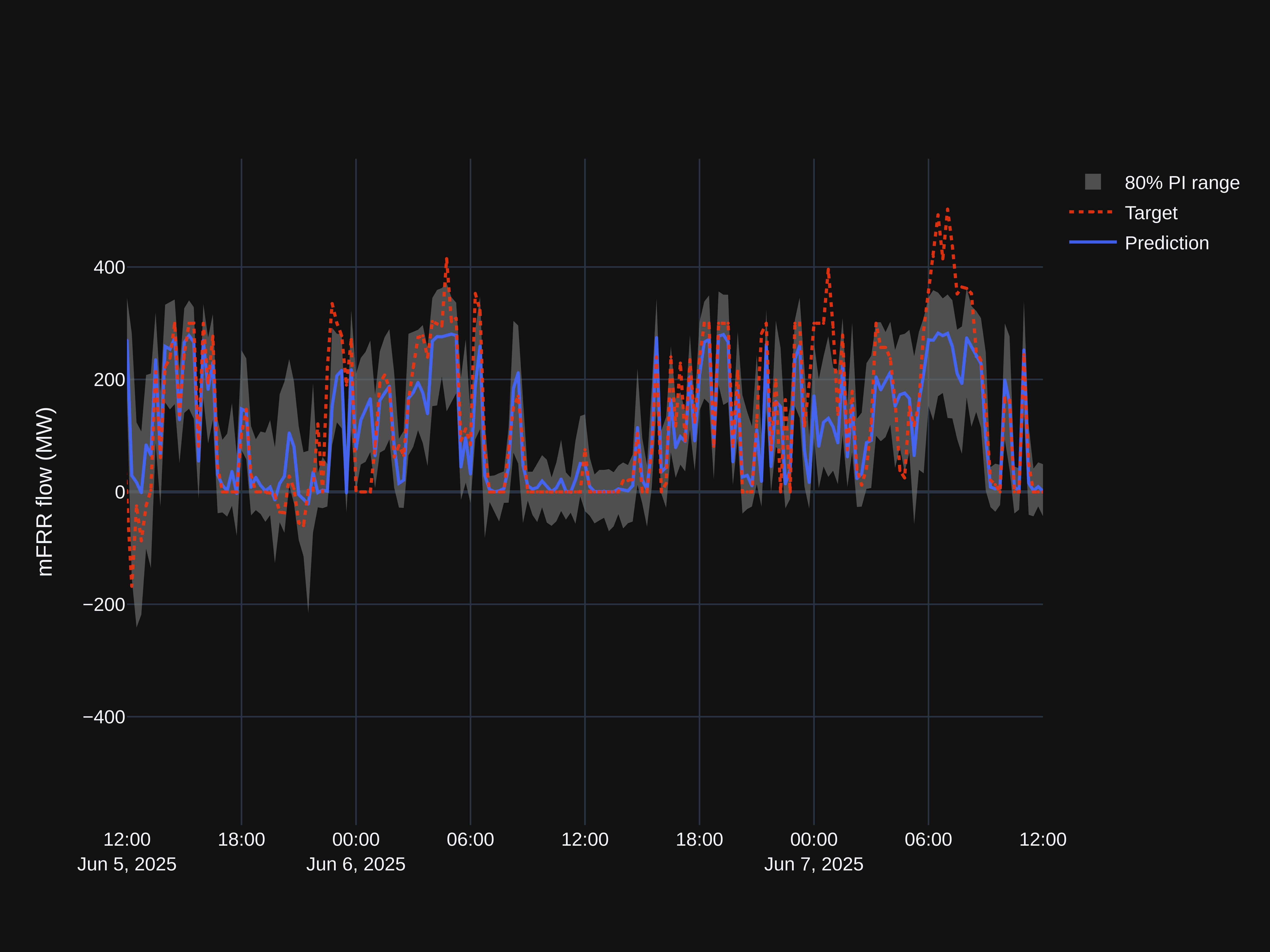
Let’s see how an 80% PI formed from the predictions of two GBT models trained on $\tau = 0.1$ and $\tau = 0.9$ looks. We’ll be using LightGBM which does leaf-wise tree growth.

This PI band looks very different from the ones we have seen so far. Its width is clearly feature-dependent, and it’s highly asymmetric in places. The fact that one PI bound often lands at 0 looks peculiar, but makes some sense given the fact that the direction of flow can often be determined with much higher confidence than the magnitude of the flow. The PI does cover regions that are outside the ATC band and therefore impossible, but not as often as with previous methods.

The empirical coverage is 80%, the mean width is 151, and the interval score is an impressive 218.

Conformalized Quantile Regression (CQR)

This method, introduced by Romano, Patterson, and Candès (2019) (PDF), combines quantile regression with conformal prediction to get the best of both worlds; the feature-dependence of quantile regression and the coverage guarantees of conformal prediction. You start with prediction intervals obtained through any regression algorithm capable of predicting specific quantiles, such as our PI from gradient boosted decision trees with pinball loss. Using conformal calibration, you then determine a constant to widen or narrow the PI width so that the coverage hits the target. It should be noted that since the target coverage is achieved by adding a non-adaptive constant, we expect the updated PI to be slightly less responsive to our features and therefore have a slightly worse local coverage, even though the marginal coverage has improved.

The algorithm, in a bit more detail:

• Split data into a training set and a calibration set.
• Train two models to predict two quantiles, $\hat{q}_ {\alpha_\text{lo}}$ and $\hat{q}_ {\alpha_\text{hi}}$, using the training set.
• Compute nonconformity scores on the calibration set using $E_i := \max{{\hat{q}_ {\alpha_\text{lo}}(x_i) – y_i, y_i – \hat{q}_ {\alpha_\text{hi}}(x_i)}}$. This score measures how much the interval would need to expand (positive) or could shrink (negative) to place the observation right at the interval boundary.
• We then find $q$, the $(1-\alpha)$-th quantile of these scores, where $(1-\alpha)$ is the desired coverage. (A finite-sample correction can be applied, meaning we use the $(1-\alpha)\left(1 + \frac{1}{|I_\text{calib}|}\right)$-th empirical quantile, where $|I_\text{calib}|$ is the number of scores)
• Given new input data, we can determine the updated prediction interval $[\hat{q}_ {\alpha_\text{lo}}(x_\text{new}) – q, \hat{q}_ {\alpha_\text{hi}}(x_\text{new}) + q]$

In our case, the actual coverage of PIs from the gradient boosted decision trees with pinball loss are already very close to the target coverage, so applying CQR is not likely to improve the results meaningfully. In fact, the coverage worsens slightly when measured on our test set, from 80.2% to 81.3%, likely due to chance difference between the calibration set and the test set. There might still be reason to include the calibration as a safeguard against future miscoverage.

The PI band shown below looks indistinguishable from the one generated with gradient boosted trees, but has in fact a constant 2 MW margin added.

On our test set, the mean interval width is 155 MW (up from 151 MW from GBT without conformal). The interval score is 218.4 (up from 218.1).

Bayesian Neural Networks (BNN)

In a Bayesian neural network, the weights and biases are represented as probability distributions instead of scalars. These distributions must be given a prior, and then undergo Bayesian updating based on our data.

We can think of a Bayesian net as a function $f(x, \theta)$, where $\theta$ are the weights and biases. The output is not a single prediction, but a distribution over possible outputs, called the posterior predictive distribution:

$$ p(y \mid x,\mathcal{D}) = \int p(y \mid x, \theta)\ p(\theta \mid \mathcal{D}) \ d\theta $$

Where:

• $\mathcal{D}$ is our training data
• $x$ is a feature vector with the new data
• $p(y \mid x, \theta)$ is the likelihood function with the probability of observing $y$ given $x$ with some $\theta$ drawn from the distribution of weights and biases
• $p(\theta \mid \mathcal{D}) = \frac{p(\mathcal{D} \mid \theta), p(\theta)}{p(\mathcal{D})}$ is the posterior of our weights and biases given the training data $\mathcal{D}$

There’s no closed form solution for the posterior predictive distribution $p(y \mid x,\mathcal{D})$. Actually, calculating the marginal data likelihood $p(\mathcal{D})$ is difficult alone, as it involves integrating over the entire weight space. We therefore have to approximate. Several methods are available, including Markov Chain Monte Carlo (MCMC) and Variational Inference (VI). MCMC involves sampling from the posterior $p(\theta \mid \mathcal{D})$ in order to estimate the predictive distribution $p(y \mid x,\mathcal{D})$, while with VI we instead approximate the posterior with a simpler distribution.

We’ve talked about how a BNN can output a predictive distribution, represented as one or more parameters. But we want a prediction interval. To get a PI from our distribution we generate a number of predictions, and take empirical quantiles of these, to form our upper and lower PI bounds, as well as our point predictions.

When using a BNN, there are several choices that have to be made. In addition to the choices one always have to make when using a neural network, a Bayesian net requires us to decide:

• Prior for the weights: Usually a simple mean-centered, independent Gaussian, acting as a form of regularization.
• The likelihood function (the form, not the parameters). This choice is an important one, as it encodes the possible values we think $y$ can take given $x$ and $\theta$. If we for example choose Gaussian, our model won’t be able to give us an asymmetric posterior predictive distribution (other than the asymmetry that might arise when integrating over the weight posteriors).
• What parameters of the likelihood function should be conditional on $x$ vs. unconditional and global. We should have heads corresponding with the conditional parameters. So if we choose an asymmetric Laplace for the likelihood, and we want all three parameters $\mu$, $b$ and $\kappa$ to be conditional on $x$, our network should have three heads, one for each. The variance of each output across weight samples captures the epistemic uncertainty, while the aleatoric uncertainty is modeled by the parameter $b$ itself.

Let’s see how BNN performs on our problem. An exhaustive search over all the possible choices is not feasible, but we’ll try a few different configurations, partially guided by our intuition.

Let’s start simple, with a Gaussian likelihood function where only $\mu(x)$ is conditional on $x$ while $\sigma$ is a global (but learned) constant. Our weight prior will be $\mathcal{N}(0, \sigma_\text{prior}^2 \cdot \mathbb{I})$, where $\sigma_\text{prior} = 0.6 \sqrt{2/\text{fan-in}}$ (this is called He-initialization, or at least it would be if it wasn’t for the scaling factor 0.6). We’ll have one hidden layer with 64 units. MCMC will be used for the approximation of the predictive distribution.

NB: All previous methods generated a PI on top of our existing point estimate, the one presented in the section titled “Data”, coming from our gradient boosted trees. But since BNNs naturally provide a point estimate as well as a PI, and since it wouldn’t make much sense to combine the point estimate from GBT with the PIs of BNN, all plots in this section will show the BNN point estimate.

Our PIs appear more or less constant in width and centered around our prediction (the small variability in width is due to randomness in the sampling process). The inability of the model to capture the feature-dependent nature of the actual prediction error is not surprising given our likelihood function with its global $\sigma$.

On the full test set we get an average PI width of 220 MW, an actual coverage of 80%, and an interval score of 318. The MAE of the new point predictions is 67 MW (GBT achieves about 49 MW).

Given the fact that our target is often conditionally heteroscedastic and asymmetric, let’s instead use an asymmetric Laplace distribution as our likelihood function. All the three parameters of the distribution will be feature-dependent via separate network heads. We’ll use the same architecture and weight prior as before, but we’ll switch out MCMC for VI (mainly for a ~ 20x speedup of the training).

We can now see clear signs of feature-dependence in the PI, both its width and asymmetry around the point prediction. It still covers regions that are impossible at times, though. And on the larger test set, the improvement in interval score is not as significant as we might expect from the plot, down from 318 to 308. The coverage is 76%, and the average width is 180. The MAE is 66 MW.

This is a bit disappointing. To understand why this highly flexible model, now capable of outputting a conditionally asymmetric predictive distribution, doesn’t perform better than this, we need to remember how the likelihood is used. The posterior predictive distribution is a sort of weighted mixture of likelihood functions across the posterior over $\theta$. Actually, we can imagine the predictive distribution as an averaging of many likelihood functions coming from traditional neural nets, all with different weights, instead of a single Bayesian one. This averaging gives us something fairly symmetric, even if the individual likelihood functions aren’t. In other words: The epistemic uncertainty (uncertainty about model weights) “washes out” the aleatoric uncertainty (the unpredictability of our data). That’s at least a likely partial explanation. We should also remember that this is a parametric approach, and as we briefly discussed earlier, our data likely isn’t amenable to such approaches. Even the relatively flexible likelihood function we have chosen can’t really model the situation where values “pile up” at a hard cap, for example.

Other Methods

For completeness, we’ll briefly mention some methods that didn’t make the cut. They are either untested or not tested thoroughly enough that I felt comfortable including the results in the main body of this blog post.

Linear Quantile Regression (LQR)

Linear quantile regression is similar to OLS, but optimizes pinball loss instead of squared error, allowing it to target specific quantiles. Given the non-linear relationships in our data, this is unlikely to perform well. LQR was briefly tested during early experimentation, giving an interval score of 269, though that number likely isn’t directly comparable to the other scores here due to later feature engineering and the use of a slightly different test set.

Gaussian Process Regression (GPR)

This topic would benefit from a longer introduction, but this will have to suffice: GPR does Bayesian inference, but over functions rather than parameters. We pick a prior that encodes our belief about what these functions look like via a “kernel function”. The GP assumes any finite set of $y$s (or to be precise, the latent function values $f(x)$, i.e. $y$ without noise) is a multivariate Gaussian where the covariances between outputs are determined by the kernel (whose parameters is the thing that is learned), capturing how similar $x$s yield similar $y$s. GPR provides a full predictive distribution $P(y|x)$ with natural uncertainty quantification. Not tested on our problem.

Mondrian Forests

A Mondrian forest is an ensemble of Mondrian trees that can output both mean predictions and uncertainty estimates. They are like random forests but with a probabilistic interpretation and online learning capabilities. Not tested.

Ensemble Forecasting

Rather than an ensemble of models, this involves running a single model multiple times with perturbed inputs to capture sensitivity to input uncertainty. Relevant if input features themselves are uncertain, but doesn’t directly address conditional heteroscedasticity.

Quantile Regression Averaging (QRA)

QRA combines point forecasts from multiple models using quantile regression. The quantile of interest is modeled as a linear combination of the individual forecasts. Useful when you have several decent point forecasters and want to produce calibrated prediction intervals. Can be sensitive to multicollinearity among forecasts. This method was briefly tested, but only with two underlying forecasters (GBT and a feedforward neural network), which is likely too few. That’s one of the challenges with this method: it requires training multiple (ideally good) models, each different enough from the others to provide useful information and avoid multicollinearity. Despite the limited number of base forecasters, we still obtained a decent interval score of 242, suggesting this approach may warrant further investigation.

Comparison

Let’s gather our results and observations, and compare.

Method	Mean width (MPIW)	Actual coverage (PICP)	Interval score
Bootstrapped In-Sample Residuals	146	74%	307
Bootstrapped Out-of-Sample Residuals	175	80%	301
Bootstrapped Binned Residuals	153	78%	301
Bootstrapped Rolling Window Residuals	148	56%	413
Conformal Prediction	175	80%	300
Conformal (Residual Normalized)	155	78%	269
GBT with Pinball Loss	151	80%	218
Conformalized Quantile Regression	155	81%	218
BNN (Gaussian Likelihood)	220	80%	318
BNN (Asymmetric Laplace)	180	76%	308

In terms of coverage, most methods hit fairly close to the target. Bootstrapped Rolling Windows Residuals is the outlier. Its miscoverage is not really surprising given how it involves sampling from residuals with the false assumption of exchangeability. That Bootstrapped In-Sample Residuals has a too low coverage is also as expected, our in-sample residuals will almost always be smaller than the out-of-sample residuals due to overfitting.

Several of the methods give PIs with an relatively small mean width, in the 146 – 155 range, yet performs poorly when measured using the interval score.

Let’s visualize the interval scores in increasing order.

We can declare GBT with Pinball Loss the winner, with it’s conformalized cousin right behind. Interestingly, the BNNs are amongst the worst-performing, despite being quite sophisticated.

Final Adjustments

While our best performing PI is impressive, we saw that it occasionally covers regions outside the ATC band. What if we simply clamp the PI band down to the ATC, removing this problem altogether? In the plot below, we have done just that. Comparing this with the unclamped PI, we see a narrowing at that central region where there was no ATC in the import direction (positive values).

With clamping, our coverage is unchanged at 80% (as expected, the removed region is outside the ATC and therefore can’t hold any values). The mean width is reduced to 147 (down from 151), and the interval score becomes 214 (down from 218).

We’ve talked a lot about the ATC in this blog post, and we just saw how clamping our PI to the ATC bounds improved our metrics. So some readers might at this point be asking: If the ATC is so informative, why not just use the ATC band in place of a PI band? How much is the ML model actually giving us compared to the ATC alone? Well, interpreting the ATC as our PI would give us an actual coverage of 100% (since the mFRR flow must always be in the ATC band), an interval score of 304, and a mean width of 304. This width is more than twice the one from the winner, and using this to inform the scenarios in the bottleneck management system would result in an unnecessarily conservative behavior and increased system regulation costs. So while the ATC is important, it’s clearly not the whole picture. We can see the difference in width between our best PI and the ATC exemplified in the plot below.

Concluding Thoughts

We set out to find a probabilistic forecasting method suited to our specific problem: mFRR flow with its hard constraints, conditional heteroscedasticity, and asymmetric uncertainty. Here are our key takeaways:

• Quantile regression with gradient boosted trees was the clear winner. It naturally captures feature-dependent uncertainty and asymmetry without strong distributional assumptions.
• Non-parametric methods outperformed parametric ones. Our data’s hard caps, heteroscedasticity and complex relationships made parametric assumptions (Gaussian errors, smooth functions) a poor fit.
• Metrics matter. If we were looking at width only, we might conclude that Bootstrapped Rolling Window Residuals is well suited. Similarly, if we were looking at coverage alone, conformal prediction and the BNN with a Gaussian Likelihood would be the winners. But these metrics don’t tell the whole story. We can, after all, achieve a perfect coverage with a PI formed by two horizontal lines, simply by moving these lines up and down until the desired fraction lies between them. Strictly proper scoring rules like the interval score or continuous ranked probability score (CRPS), on the other hand, capture more of what we actually care about: narrow intervals that still achieve good conditional coverage. Still, depending on what matters for your use case, you might have to look at multiple metrics when comparing methods.
• Domain knowledge can improve results. Clamping the PI to the ATC bounds, a simple post-processing step using our knowledge of physical constraints, improved our interval score slightly, with no downside.

It is of course important to remember that a different problem may have different characteristics than ours, and what worked here might not be the best fit for you. If your data is more homoscedastic, or if marginal coverage matters more than conditional coverage, conformal prediction might be a better choice. If changes are slow relative to your sampling frequency, sampling from a rolling window could work well. Whatever your problem looks like, we hope this discussion has helped illuminate the tradeoffs involved, and given you some ideas for what to look for when choosing a method.