Load forecasting, also referred to as consumption prognosis, combines techniques from machine learning with knowledge of the power system. It’s a task that fits like a glove for the Data Science team at Statnett and one we have been working on for the last months.

We started with a three week long Proof of Concept to see if we could develop good load forecasting models and evaluate the potential of improving the models. In this period, we only worked on offline predictions, and evaluated our results against past power consumption.

The results from the PoC were good, so we were able to continue the work. The next step was to find a way to go from offline predictions to making online predictions based on near real time data from our streaming platform. We also needed to do quite a bit of refactoring and testing of the code and to make it production ready.

After a few months of work, we have managed to build an API to provide online predictions from our scikit learn and Tensorflow models, and deploy our API as a container application on OpenShift.

Good forecasts are necessary to operate a green power system

Balancing power consumption and power production is one of the main responsibilities of the National Control Centre in Statnett. A good load forecast is essential to obtain this balance.

The balancing services in the Nordic countries consist of automatic Frequency Restoration Reserves (aFRR) and manual Frequency Restoration Reserves (mFRR). These are activated to contain and restore the frequency. Until the Frequency Restoration Reserves have been activated, the inertia (rotating mass) response and system damping reduce the frequency drop below unacceptable levels.

The growth in renewable energy sources alters the generation mix; in periods a large part of the generators will produce power without simultaneously providing inertia. Furthermore, import on HVDC-lines do not contribute with inertia. Therefore, situations with large imports to the Nordic system can result in insufficient amount of inertia in the system. A power system with low inertia will be more sensitive to disturbances, i.e. have smaller margins for keeping frequency stability.

That is why Statnett is developing a new balancing concept called Modernized ACE (Area Control Error) together with the Swedish TSO Svenska kraftnät. Online prediction of power consumption is an integral part of this concept and is the reason we are working on this problem.

Can we beat the existing forecast?

Statnett already has load forecasts. The forecasts used today are proprietary software, so they are truly black box algorithms. If a model performs poorly in a particular time period, or in a specific area, confidence in the model can be hard to restore. In addition, there is a need for predictions for longer horizons than the current software is providing.

We wanted to see if we could measure up to the current software, so we did a three week stunt, hacking away and trying to create the best possible models in the limited time frame. We focused on exploring different features and models as well as evaluating the results to compare with the current algorithm.

At the end of this stunt, we had developed two models: one simple model and one complex black box model. We had collected five years of historical data for training and testing, and used the final year for testing of the model performance.

Base features from open data sources

The current models provide predictions for the next 48 hours for each of the five bidding zones in Norway. Our strategy is to train one model for each of the zones. All the data sources we have used so far are openly available:

• weather observations can be downloaded from the Norwegian Meteorological Institutes’s Frost API. We retrieve the parameters wind speed and air temperature from the observations endpoint, for specific weather stations that we have chosen for each bidding zone.
• weather forecasts are available from the Norwegian Meteorological Institute’s thredds data server. There are several different forecasts, available as grid data, along with further explanation of the different forecasts and the post processing of parameters. We use the post processed unperturbed member (the control run) of the MetCoOp Ensemble Prediction System (MEPS), the meps_det_pp_2_5km-files. From the datasets we  extract wind speed and air temperature at 2 m height for the closest points to the weather stations we have chosen for each bidding zone.
• historical hourly consumption per bidding area is available from Nord Pool

Among the features of the models were:

• weather observations and forecasts of temperature and wind speed from different stations in the bidding zones
• weather parameters derived from observations and forecasts, such as windchill
• historical consumption and derived features such as linear trend, cosine yearly trend, square of consumption and so on
• calendar features, such as whether or not the day is a holiday, a weekday, the hour of the day and so on

Prediction horizon

As mentioned, we need to provide load forecasts for the next 48 hours, to replace the current software. We have experimented with two different strategies:

• letting one model predict the entire load time series
• train one model for each hour in the prediction horizon, that is one model for the next hour, one model for two hours from now and so on.

Our experience so far is that one model per time step performs better, but of course it takes more time to train, and is more complex to handle. This explodes if the frequency of the time series is increased or the horizon is increased: perhaps this will be too complex for a week ahead load forecast, resulting in 168 models for each bidding zone.

Choosing a simple model for correlated features

We did some initial experiments using simple linear regression, but quickly experienced the problem of bloated weights: The model had one feature with a weight of about one billion, and another with a weight of about minus one billion. This resulted in predictions in the right order of magnitude, but with potential to explode if one feature varied more than usual.

Ridge regression is a form of regularization of a linear regression model, which is designed to mitigate this problem. For correlated features, the unbiased estimates for least squares linear regression have a high variance. This can lead to bloated weights making the prediction unstable.

In ridge regression, we penalize large weights, thereby introducing a bias in the estimates, but hopefully reducing the variance sufficiently to produce reliable forecasts. In linear least squares we find the weights minimizing the error. In ridge regression, we penalize the error function for having large weights. That is we add a term in proportion to the sum square of the weights x₁ and x₂ to the error. This extra penalty can be illustrated with circles in the plane, the farther you are from the origin, the bigger the penalty.

For our Ridge regression model, we used the Ridge class from the Python library scikit learn.

Choosing a neural network that doesn’t forget

Traditional neural networks are unable to remember information from earlier time steps, but recurrent neural networks (RNNs) are designed to be able to remember from earlier time steps. Unlike the simpler feed-forward networks where information can only propagate in one direction, RNNs introduce loops to pick up the information from earlier time steps. An analogy for this is being able to see a series of images as a video, as opposed to considering each image separately. The loops of the RNN is unrolled to form the figure below, showing the structure of the repeating modules:

In practice, RNNs are only able to learn dependencies from a short time period. Long short-term memory networks, LSTMs are a type of RNNs that use the same concept of loops as RNNs, but the value lies in how the repeating module is structured.

One important distinction from RNNs is that the LSTM has a cell state, that flows through the module only affected by linear operations. Therefore, the LSTM network doesn’t “forget” the long term dependencies.

For our LSTM model we used the Keras LSTM layer.

For a thorough explanation of LSTM, check out this popular blog post by Chris Olah: Understanding LSTMs.

Results

To evaluate the models, we used mean absolute percentage error, MAPE, which is a common metric used in load forecasting. Our proof of concept models outperformed the current software when we used one year of test data, reducing the MAPE by 28% on average over all bidding zones in the forecasts.

We thought this was quite good for such a short PoC, especially considering that the test data was an entire year. However, we see that for the bidding zone NO1 (Østlandet), where the power consumption is largest, we need to improve our models.

How to evaluate fairly when using weather forecasts in features

We trained the models using only weather observations, but when we evaluated performance, we used weather forecasts for time steps after the prediction time. In the online prediction situation, observations are available for the past, but predictions must be used for the future. To compare our models with the current model, we must simulate the same conditions.

We have also considered training our model using forecasts, but we only have access to about a year of forecasts, therefore we have chosen to train on observations. Another possible side effect of training on forecasts, is the possibility of learning the strengths and weaknesses of a specific forecasting model from The Norwegian Meteorological Institute. This is not desirable, as we would have to re-learn the patterns when a new model is deployed. Also, the model version (from the Meteorological Institute) is not available as of now, so we do not know when the model needs re-training.

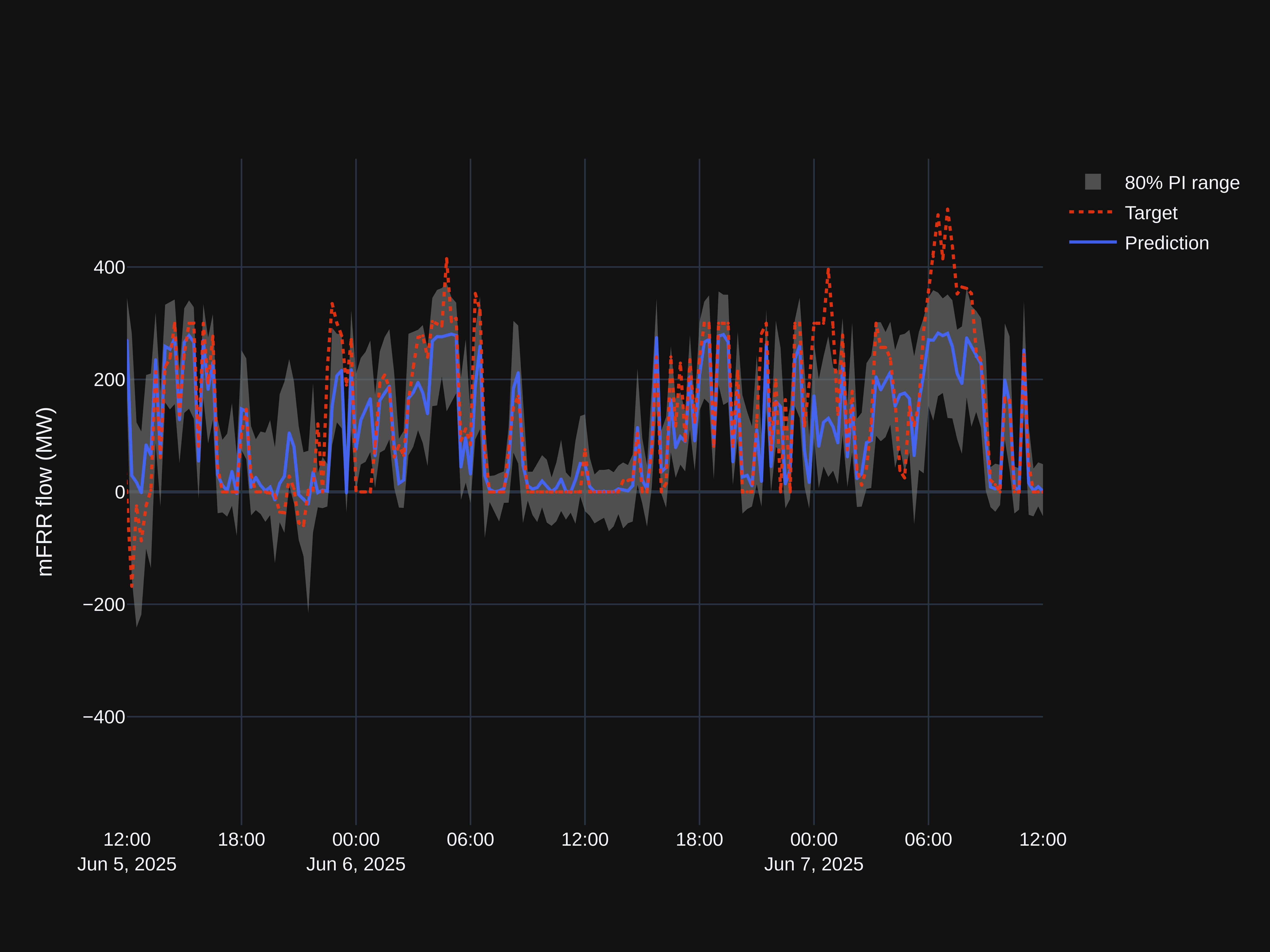
Our most recent load forecast

By now we have made some adjustments to the model, and our forecasts for NO1 from the LSTM model and Ridge regression model are shown below. Results are stored in a PostgreSQL database and we have built a Grafana dashboard visualizing results.

How to deploy real time ML models to OpenShift

The next step in our development process was to create a framework for delivering online predictions and deploy it. This also included refactoring the code from the PoC. We worked together with a development team to sketch out an architecture for fetching our data from different sources to delivering a prediction. The most important steps so far have been:

• Developing and deploying the API early
• Setting up a deployment pipeline that automatically deploys our application
• Managing version control for the ML models

Develop and deploy the API early

“API first” development (or at least API early, as in our case) is often referenced as an addition to the twelve-factor app concepts, as it helps both client and server side define the direction of development. A process with contracts and requirements sounds like a waterfall process, but our experience from this project is that in reality, it supports an agile process as the requirements are adapted during development. Three of the benefits were:

• API developers and API users can work in parallel. Starting with the API has let the client and server side continue work on both sides, as opposed to the client side waiting for the server side to implement the API. In reality, we altered the requirements as we developed the API and the client side implemented their use of it. This has been a great benefit, as we have uncovered problems, and we have been able to adjust the code early in the development phase.
• Real time examples to end users. Starting early with the API allows us to demonstrate the models with real time examples to the operators who will be using the solution, before the end of model development. The operators will be able to start building experience and understanding of the forecasts, and give feedback early.
• Brutally honest status reports. Since the results of the current models are available at any time, this provides a brutally honest status report of the quality of the models for anyone who wants to check. With the models running live on the test platform, we have some time to discover peculiarities of different models that we didn’t explore in the machine learning model development phase, or that occur in online prediction and not necessarily in the offline model development.

Separate concerns for the ML application and integration components

Our machine learning application provides an API that only performs predictions when a client sends a request with input data. Another option could be to have the application itself fetch the data and stream the results back to our streaming platform, Kafka.

We chose not to include fetching and publishing data inside our application in order to separate concerns of the different components in the architecture, and hopefully this will be robust to changes in the data sources.

The load forecasts will be extended to include Sweden as well. The specifics of how and where the models for Sweden will run are not decided, but our current architecture does not require the Swedish data input. Output is written back to Kafka topics on the same streaming platform.

The tasks we rely on are:

• Fetching data from the different data sources we use. These data are published to our Kafka streaming platform.
• Combine relevant data and make a request for a forecast when new data is available. A java application is scheduled each hour, when new data is available.
• Make the predictions when requested. This is where the ML magic happens, and this is the application we are developing.
• Publish the prediction response for real time applications. The java application that requests forecasts also publishes the results to Kafka. We imagine this is where the end-user applications will subscribe to data.
• Store the prediction response for post-analysis and monitoring.

How to create an API for you ML models

Our machine learning application provides an API where users can supply the base features each model uses and receive the load forecast for the input data they provided. We created the API using the Python library Flask, a minimal web application framework.

Each algorithm runs as a separate instance of the application, on the same code base. Each of these algorithm instances has one endpoint for prediction. The endpoint takes the bidding zone as an input parameter and routes the request to the correct model.

Two tips for developing APIs

• Modularize the app and use blueprint with Flask to prevent chaos. Flask makes it easy to quickly create a small application, but the downside is that it is also easy to create a messy application. After first creating an application that worked, we refactored the code to modularize. Blueprints are templates that allow us to create re-usable components.
• Test your API using mocking techniques. As we refactored the code and tried writing good unit tests for the API, we used the mock library to mock out objects and functions so that we can separate which functionality the different tests test and run our tests faster.

Where should derived features be calculated?

We have chosen to calculated derived features (i.e. rolling averages of temperature, lagged temperature, calendar features and so on) within the model, based on the base features as input data. This could have been outside of the models, for example by the java application that integrates the ML and streaming, or by the Kafka producers. There are two main reasons why we have chosen to keep these calculations inside our ML API:

• The feature data is mostly model specific, and lagged data causes data duplication. This is not very useful for anyone outside of the specific model, and therefore it doesn’t make sense to create separate Kafka topics for these data or calculate them outside of the application.
• Since we developed the API at an early stage, we had (and still have) some feature engineering to do, and we did not want to be dependent on someone else to provide all the different features that we wanted to explore before we could deploy a new model.

Class hierarchy connects general operators to specific feature definitions

The calculations of derived features are modularized in a feature operator module to ensure that the same operations are done in the same way everywhere. The link that applies these feature operators to the base features is implemented using class methods in a class hierarchy.

We have created a class hierarchy as illustrated in the figure above. The top class, ForecastModels, contains class methods for applying the feature operators to the input data in order to obtain the feature data frame. Which base features and which feature operators we want to be applied to the features are specified in the child class.

The child classes at the very bottom, LstmModel and RidgeRegression, inherit from their respective Keras and scikit learn classes as well, providing the functionality for the prediction and training.

As Tensorflow models have a few specific requirements, such as normalising the features, this is implemented as a class method for the class TensorFlowModels. In addition, the LSTM models require persisting the state for the next prediction. This is handled by class methods in the LstmModel class.

Establish automatic deployment of the application

Our deployment pipeline consists of two steps, which run each time we push to our version control system:

• run tests
• deploy the application to the test environment if all tests pass

We use GitLab for version control, and have set up our pipeline using the integrated continuous integration/continuous deployment pipelines. GitLab also integrates nicely with the container platform we use, OpenShift, allowing for automatic deployment of our models through a POST request to the OpenShift API, which is part of our pipeline.

Automatic deployment has been crucial in the collaboration with the developers who make the integrations between the data sources and our machine learning framework, as it lets us test different solutions easily and get results of improvements immediately. Of course, we also get immediate feedback when we make mistakes, and then we can hopefully fix it while we remember what the breaking change was.

How we deploy our application on OpenShift

Luckily, we had colleagues who were a few steps ahead of us and had just deployed a Flask application to OpenShift. We used the source to image-build strategy, which builds a Docker image from source code, given a git repository. The Python source to image image builder is even compatible with the environment management package we have used, Pipenv, and automatically starts the container running the script app.py. This allowed us to deploy our application without any adaptions to our code base other that setting an environment variable to enable Pipenv. The source-to-image strategy was perfect for the simple use case, but we are now going towards a Docker build strategy because we need more options in the build process.

For the LSTM model, we also needed to find a way to store the state, independently of deployments of the application. As a first step, we have chosen to store the states as flat files in a persistent storage, which is stored independently of new deployments of our application.

How do we get from test to production?

For deployment from the production to the test environment, we will set up a manual step after verifying that everything is working as expected in the test environment. The plan as of now is to publish the image running in the test environment in OpenShift to Artifactory. Artifactory is a repository manager we use for hosting internally developed Python packages and Docker images that our OpenShift deployments can subscribe to. The applications running in the OpenShift production environment can then be deployed from the updated image.

Flask famously warns us not to use it in production because it doesn’t scale. In our setting, one Flask application will receive one request per hour per bidding zone, so the problems should not be too big. However, if need be, we plan to use the Twisted web server for our Flask application. We have used Twisted previously when deploying a Dash web application, which is also based on Flask, and thought it worked well without too much effort.

Future improvements

Choosing the appropriate evaluation metric for models

In order to create a forecast that helps the balancing operators as much as possible, we need to optimize our models using a metric that indicates their need. For example, what is most important: Predicting the level of the top load in the day, or predicting the time the top load occurs on? Is it more important to predict the outliers correctly or should we focus on the overall level? This must be decided in close cooperation with the operators, illustrating how different models perform in the general and in the special case.

Understanding model behavior

Understanding model behavior is important both in developing models and to build trust in a model. We are looking into the SHAP framework, which combines Shapley values and LIME to explain model predictions. The framework provides plots that we think will be very useful for both balancing operators and data scientists.

Including uncertainty in predictions

There is of course uncertainty in the weather forecasts and the Norwegian Meteorological Institute provides ensemble forecasts. These 10 forecasts are obtained by using the same model, but perturbing the initial state, thereby illustrating uncertainty in the forecast. For certain applications of the load forecast, it could be helpful to get an indication of the uncertainty in the load forecast, for example by using these ensemble forecast to create different predictions, and illustrating the spread.