

On June 17th 2024, we sat down in randomly assigned teams of three, where everyone from the section leader to summer interns participated. We were presented with data, a problem description, and a submission deadline. In only six frantic hours, who among us could best predict how the homes and businesses in eastern Norway would consume power over the course of 4 months? And how would our best forecasts stack up against commercially available consumption forecasts?
The Challenge
The task was simple: Forecast power consumption in NO1 (one of Norway’s 5 price areas, located in the eastern part of the country) for every hour from January 1st to April 30th, 2024. We were allowed to use historical power consumption data during training, but only up to and including 2023. During inference, we could use historical consumption data from 2024, but only up to 6 am on the day before the forecast horizon. This restriction was in place to simulate the real-world scenario where we need to publish our forecasts for the day ahead.
In addition, we were given weather data for 49 locations in the NO1 area, including observations of temperature, wind speed, wind direction, cloud coverage, air pressure, humidity, and precipitation. For the sake of the exercise, we treated historical weather data as though it were forecast data.
No other data were to be used, but we were allowed to extract and engineer additional features from the provided data, including dates and times.
The predictions were to be submitted through Kaggle, where the score would be automatically calculated as the root-mean-squared error (RMSE). The RMSE was evaluated for every hour from January 1st 00:00 through April 30th 23:00.
The Solutions
After the teams had hacked away at the problem for six hours, we gathered to declare the winner and share some insights about what worked and what didn’t. It was fascinating to see the diverse techniques deployed by different teams. Some used the somewhat simple ridge regression (linear regression with an extra term in the loss function that penalizes high model coefficients). Others used more flexible models like boosted decision tree ensembles and neural networks. Some employed ensembles consisting of both complex neural nets and simple linear models. And some teams experimented with 24 models, one for each hour of the day, while others used a multi-output regressor to predict all 24 hours for a given day at once.
Feature engineering approaches varied as well. Some teams created simple features based on the date and time of day, such as the hour of the day, the day of the week, and the month, represented as basic integers, and perhaps an extra is_holiday feature indicating holidays. Others used more complex representations, like individual one-hot encoded variables for each holiday or sine and cosine transformations of the day of the year and hour of the day.
All teams used lagged power consumption data in some form, but again, the solutions differed in their details. For instance, some only provided the model with consumption data from a very few points in time that seem especially relevant, like the consumption at the same time of day one week prior. Others included much more consumption data, like the history 48 hours before the day-ahead prediction time point, in the hope that the model would pick up on useful trends and patterns.
Here’s an example of the code used by one of the teams. It uses XGBRegressor, a regressor that can output 24 predictions at once. This is an example of the decision tree ensemble mentioned earlier. Overfitting seemed to be an issue for this model, so a number of techniques were used to prevent it, including early stopping and the reg_alpha passed to the constructor, which scales the L1 regularization term to penalize large coefficients.
from pathlib import Path
import numpy as np
import pandas as pd
import seaborn as sns
from holidays import country_holidays
from matplotlib import pyplot as plt
from sklearn.metrics import root_mean_squared_error
from sklearn.model_selection import train_test_split
from sklearn.preprocessing import MinMaxScaler
from xgboost import XGBRegressor, plot_importance

# https://kart.ssb.no/befolkning
LOCATION_WEIGHTS = {"Asker": 1, "Askim": 1, "Ås": 1, "Beitostølen": 1, "Bekkestua": 1, "Blindern": 1, "Dokka": 1, "Drammen": 3, "Drøbak": 1, "Eidsvoll": 1, "Elverum": 2, "Fagernes": 1, "Fetsund": 1, "Flisa": 1, "Fredrikstad": 2, "Gjøvik": 2, "Halden": 1, "Hamar": 3, "Hønefoss": 2, "Jessheim": 1, "Kongsberg": 2, "Kongsvinger": 1, "Koppang": 1, "Lambertseter": 1, "Lillehammer": 1,  "Lillestrøm": 1, "Moss": 5, "Mysen": 1, "Nesodden": 1, "Notodden": 2, "Oslo": 20, "Otta": 1, "Rakkestad": 1, "Rena": 1, "Ringebu": 1, "Rotnes": 1, "Røros": 1, "Sarpsborg": 7, "Ski": 1, "Sørumsand": 1, "Spydeberg": 1, "Stovner": 1, "Sætre": 1, "Trysil": 1, "Tynset": 1, "Veggli": 1, "Vestby": 1, "Vikersund": 1, "Vinstra": 1}


def load_weather() -> tuple[pd.DataFrame, pd.DataFrame]:
    """Load weather data for all 49 locations and calculate weighted mean."""
    weather_list = []
    for file_path in Path("../data/weather").glob("*.parquet"):
        weather = pd.read_parquet(file_path)
        cols = [
            "air_temperature_2m",
            # 'air_pressure_at_sea_level',
            # 'relative_humidity_2m',
            "cloud_area_fraction",
            # 'precipitation_amount',
            "wind_speed_10m",
            # 'wind_direction_10m'
        ]
        weather = weather.loc[:, cols]
        weather = weather.add_prefix(file_path.stem + "_")
        weather_list.append(weather)

    weather_df = pd.concat(weather_list, axis=1)

    weighted_mean_weather = pd.DataFrame(index=weather_df.index)
    for measurement in {col.split("_", 1)[1] for col in weather_df.columns}:
        total_weight = sum(LOCATION_WEIGHTS.values())
        weighted_sum = sum(
            weather_df[f"{loc}_{measurement}"] * LOCATION_WEIGHTS[loc]
            for loc in LOCATION_WEIGHTS
            if f"{loc}_{measurement}" in weather_df.columns
        )
        weighted_mean_weather[measurement] = weighted_sum / total_weight

    return weather_df, weighted_mean_weather


def scale_weather(mean_weather_df: pd.DataFrame) -> pd.DataFrame:
    x_scaled = MinMaxScaler().fit_transform(mean_weather_df.values)
    return pd.DataFrame(x_scaled, index=mean_weather_df.index, columns=mean_weather_df.columns)


def load_train_and_test_target() -> pd.DataFrame:
    """Load consumption data for training and testing."""
    train_raw = pd.read_parquet("../data/train_target.parquet")
    train_raw = train_raw.tz_convert(None)
    train_raw = train_raw.rename(columns={"cleaned": "cons"})

    test_raw = pd.read_csv("../data/test_target.csv", index_col="id")
    test_raw.index = pd.date_range(start="2024-01-01", periods=len(test_raw), freq="h")
    test_raw = test_raw.rename(columns={"target": "cons"})

    return pd.concat([train_raw, test_raw])


def make_daily(df: pd.DataFrame) -> pd.DataFrame:
    """Resample time series to daily frequency.

    Returns:
        A DataFrame with daily frequency and 24 columns for each observation.
    """
    df = df.sort_index()
    df = df[~df.index.duplicated(keep="first")]
    complete_date_rng = pd.date_range(start=df.index.min(), end=df.index.max(), freq="h")
    df = df.reindex(complete_date_rng)
    df = df.interpolate()
    df = df.dropna()
    daily_df = df.resample("D").apply(lambda x: x.values.tolist())
    transformed_df = pd.DataFrame(index=daily_df.index)
    for hour in range(24):
        for column in df.columns:
            new_column_name = f"{column}_{hour}"
            transformed_df[new_column_name] = daily_df[column].apply(lambda x: x[hour] if len(x) > hour else None)
    return transformed_df


def add_dt_features(df: pd.DataFrame, country_code: str = "NO") -> pd.DataFrame:
    """Create date related features based on time series index with daily frequency."""
    df = df.copy()
    df["dayssincestart"] = (df.index - df.index[0]).days / (4 * 365)
    df["sindayofweek"] = np.sin(df.index.dayofweek / 7 * 2 * np.pi)
    df["cosdayofweek"] = np.cos(df.index.dayofweek / 7 * 2 * np.pi)
    for i in range(7):
        df[f"daytype_{i}"] = df.index.dayofweek == i
    df["sindayofyear"] = np.sin(df.index.dayofyear / 365 * 2 * np.pi)
    df["cosdayofyear"] = np.cos(df.index.dayofyear / 365 * 2 * np.pi)
    df["timeoffset"] = df.index.tz_localize("Europe/Oslo").map(lambda r: r.utcoffset()).astype(int) / 3.6e12
    holidays = country_holidays(country_code)
    df["is_holiday"] = df.index.to_series().apply(lambda x: 1 if x in holidays else 0)
    df["is_bridge_day"] = (
        (df["is_weekend"].shift(1, fill_value=0) | df["is_holiday"].shift(1, fill_value=0))
        & (df["is_weekend"].shift(-1, fill_value=0) | df["is_holiday"].shift(-1, fill_value=0))
        & ~(df["is_weekend"])
        & ~(df["is_holiday"])
    ).astype(int)
    return df


def add_lag_features(df: pd.DataFrame) -> pd.DataFrame:
    """Add lag features to time series."""
    df = df.copy()
    df[[f"cons-D-7-h{i}" for i in range(24)]] = df[[f"cons_{i}" for i in range(24)]].shift(7)  # One week ago
    df[[f"cons-D-2-h{i}" for i in range(24)]] = df[[f"cons_{i}" for i in range(24)]].shift(2)  # Two days ago
    df[[f"cons-D-1-h{i}" for i in range(7)]] = df[[f"cons_{i}" for i in range(7)]].shift(1)  # Yesterday util 6am
    df[[f"air_temp-D-7-h{i}" for i in range(24)]] = df[[f"air_temperature_2m_{i}" for i in range(24)]].shift(7)
    return df


def train_xgboost(X_train, y_train, X_test, y_test, use_saved=False, estimators=50) -> XGBRegressor:
    """Train XGBoost regressor on training data and return the model."""
    model_path = Path("../models/xgboost.json")
    if use_saved and model_path.exists():
        print("Using saved XGBoost model ...")
        reg = XGBRegressor()
        reg.load_model(model_path)
        return reg

    print("Training XGBoost model ...")
    reg = XGBRegressor(
        base_score=y_train["cons_8"].mean(),
        booster="gbtree",
        n_estimators=estimators,
        early_stopping_rounds=15,
        objective="reg:squarederror",
        max_depth=4,
        learning_rate=0.3,
        subsample=0.8,
        colsample_bytree=0.8,
        min_child_weight=3,
        reg_alpha=10000,
    )
    reg.fit(X_train, y_train, eval_set=[(X_train, y_train), (X_test, y_test)], verbose=10)
    reg.save_model(model_path)
    return reg


def main():
    # Preparing the data
    weather_df, unscaled_mean_weather_df = load_weather()
    mean_weather_df = scale_weather(unscaled_mean_weather_df)
    data_hourly = load_train_and_test_target()
    data_hourly = data_hourly.join(mean_weather_df)
    cons_scale = data_hourly["cons"].max()
    data_hourly["cons"] = data_hourly["cons"] / cons_scale
    data_daily = make_daily(data_hourly)

    data_daily = add_lag_features(data_daily)
    data_daily = add_dt_features(data_daily, country_code="NO")

    target_cols = [f"cons_{i}" for i in range(24)]
    feature_cols = list(data_daily.columns.difference(target_cols))
    # Scale up consumption target columns to correct scale again
    data_daily[target_cols] = data_daily[target_cols] * cons_scale

    data_submission = data_daily.loc["2024-01-01":]
    data_daily = data_daily.loc[:"2024-01-01"]

    # Test train split
    X_train_val = data_daily[feature_cols]
    Y_train_val = data_daily[target_cols]
    X_train, X_test, y_train, y_test = train_test_split(X_train_val, Y_train_val, test_size=0.25, shuffle=False)

    # Train model
    model = train_xgboost(X_train, y_train, X_test, y_test, False)

    # Plot feature importance
    plot_importance(model, max_num_features=20)
    plt.show()

    # Evaluate model
    predictions = model.predict(X_test)
    predictions = pd.DataFrame(predictions, index=y_test.index, columns=y_test.columns)

    y_test = y_test.sort_index()
    predictions = predictions.sort_index()

    fig, axes = plt.subplots(2, 2, figsize=(20, 20))
    axes = axes.flatten()
    sns.heatmap(y_test, cmap="viridis", ax=axes[0])
    axes[0].set_title("y_test")
    sns.heatmap(predictions, cmap="viridis", ax=axes[1])
    axes[1].set_title("predictions")
    sns.heatmap(y_test.subtract(predictions), cmap="viridis", ax=axes[2])
    axes[2].set_title("residuals")
    plt.tight_layout()
    plt.show()

    rmse = root_mean_squared_error(y_test, predictions)
    print(f"Root Mean Squared Error on training date range: {rmse:.2f}")

    # Train model again
    print("Training model on full dataset ...")
    model = train_xgboost(X_train_val, Y_train_val, X_test, y_test, False, model.best_iteration)

    predictions = model.predict(X_train_val)
    predictions = pd.DataFrame(predictions, index=Y_train_val.index, columns=Y_train_val.columns)
    Y_train_val = Y_train_val.sort_index()
    predictions = predictions.sort_index()
    rmse = root_mean_squared_error(Y_train_val, predictions)
    print(f"Root Mean Squared Error on full dataset: {rmse:.2f}")

    # Make final predictions for submission
    predictions = model.predict(data_submission.loc[:, feature_cols])
    predictions = pd.DataFrame(predictions, index=data_submission.index, columns=target_cols)
    output = pd.DataFrame(predictions.to_numpy().flatten()).reset_index().rename(columns={"index": "id", 0: "target"})
    output.to_csv(f"../predictions/xgboost_predictions_rmse_{rmse:.2f}.csv", index=False, header=["id", "target"])


if __name__ == "__main__":
    main()
The Winning Strategy
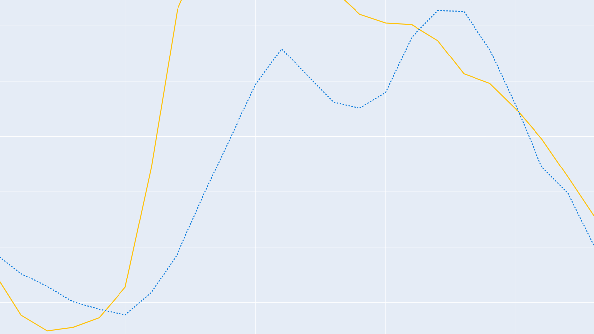
The winning team achieved an RMSE of 188.3, outperforming both an existing prognosis created by Statnett and commercial prognoses we have access to. The pediction is illustrated below. Of course, the fact that we were using weather observations instead of weather forecasts might have given us an unfair advantage.
So what was the winning strategy? The winning team used the MLPRegressor from scikit-learn, an implementation of a feedforward neural network. Applying such a flexible model capabable of learning complex relationships, and increasing the included historic data to 48 hours prior to the day-ahead predicition time-point will likely be important explanatory factors of the accuracy of the prediction. Additionally, through looking up and labelling which days were “holidays”, “weekends”, and “workdays”, these could be added to the feature matrix by one hot encoding, which produced a considerably improved forecast. Another remark made by the winning team was that they found using weather data from only one or a few highly populated locations in the data set was sometimes better than using the majority of locations. However, there was not time to fully explore the data set, and there may likely be unexplored combinations of these locations that may be even more informative. More time to fine-tune the training of the neural network and hyperparameters could possibly yield even better results.

Key Takeaways
In retrospect, we can say that the benefits the Data Science section has reaped from this exercise have been multifaceted:
- It was a fun, and intense team-building experience, where people who normally worked in different projects got to work together.
- A way to have a change of pace and perspectives compared to the ordinary work-day for many of us.
- Those who do not normally work with forecasting and/or ML models got to learn more about those activities within the group, thereby increasing the over-all group competency in these disciplines.
- The resulting ensemble of different solutions generated experience and knowledge with ML which may be implemented or used in different on-going projects within Statnett.
All-in-all, this was a fun learning experience for all who participated, and a primer for doing more similar activities in the future. If you wish to read and learn more about forecasting activities within Statnett, we refer you to the resources below:


Leave a Reply