
This summer we have had two summer interns working as part of the data science team at Statnett: Norunn Ahdell Wankel from Industrial Mathematics at NTNU and Vegard Solberg from Environmental Physics and Renewable Energy at NMBU. We asked them to look at our failure prediction models and the underlying data sources with a critical eye. They have written this blog post to document their work. At the end of the article we offer some reflections. Enjoy!
Statnett already has its own models used to forecast probability of failure due to wind or lightning on the transmission lines. If you want to know more about the lightning model and how it is used to forecast probability of failure we recommend you to have a look at some previous blog posts from April on the details of the model and how it is used. Both of the models are, however, based on another climate data source (reanalysis data computed by Kjeller vindteknikk) than what is used as input in realtime forecasting (weather forecast from Norwegian Meteorological Institute – Met). With this in mind, together with the fact that Statnett’s models have not yet been properly evaluated or challenged by other models, we aim to answer the following questions:
- How similar is the weather data from Kjeller and Met?
- How good is the model currently in use, developed by the Data Science team?
- Can we beat today’s model?
Short overlap period between the weather data from Met and Kjeller
We must have an overlap period of data from Met and Kjeller to be able to compare the differences in weather. Unfortunately, we only had four full months of overlap. This period corresponds to February 1 – May 30, 2017, for which we have hourly data for each tower along 238 transmission lines. There were only failures due to wind and none due to lightning in the overlap period. Therefore we have chosen to only focus on the wind model and hence the wind speed for the rest of this blog post.
Kjeller reports stronger wind
Kjeller gives a wind speed that on average is 0.76 m/s higher than Met in the overlap period. However, this is not the case for all lines. We get a feeling of the variation between lines by averaging the difference (Met minus Kjeller) per tower within a line and sort the difference in descending order. This is shown in the second column of the table below, from which it is clear that there is variety, and not a “trend”. The mean differences ranges from +1.55 to -2.74 m/s. Also noting that only 58 out of the 238 lines in total have a positive mean difference, the trend, if speaking of one, is that Kjeller records a higher wind speed on average for most lines.

The third and fourth columns display the number of hours in which at least one tower along a line had a wind speed above 15 m/s (i.e that the max speed over the whole line exceeded 15 m/s in that hour). Why exactly 15 m/s? Because Statnett’s model for wind failures uses this threshold, meaning that a wind speed lower than this does not affect the wind exposure and therefore not the probability of failure. We see quite a huge difference between Met and Kjeller. For 179 of the 238 lines Kjeller reported a larger number of hours than Met. To visualize the difference better we can plot the difference in number of hours the max wind speed is above 15 m/s between Met and Kjeller as a histogram, see figure below.

Clearly the histogram also shows how Kjeller reports more hours than Met for most lines. However only very few of them have an absolute difference of more than 200 hours.
Larger variance in Kjeller data
We found that Kjeller has a greater average variance within a line than Met. By finding the standard deviation at a line at each specific time point, and thereafter averaging over all times, we get the values reported in the columns “Mean std per hour”. In 199 cases Kjeller has a larger standard deviation than MET, indicating that Kjeller reports more different values along a line than Met.
Kjeller also has a higher variance throughout the whole overlap period. We calculated the standard deviation over all hours for each tower, and then found the mean standard deviation per tower along a line. The numbers are found in the columns “mean std per tower”. They tell us something about how the wind speeds for a tower tend to vary during the whole time period. It turns out that Kjeller has a higher standard deviation in 182 of the cases.
Is there any geographical trend?
Having summarized wind speeds for each line we were curious to see if there could be a geographical trend. We looked at the mean differences when grouping the transmission lines based on which region they belong to, hence either N, S or M (north, south, mid). This is illustrated in the plot below.

As seen from the plot “N” is the region that stands a bit out from the other, where Kjeller is mainly lower than Met. The spread in values is however large for all regions. Maybe another grouping of the data would have revealed stronger trends. One could for instance have investigated if there is any trend tower-wise based on latitude and longitude coordinates for each tower. What would also have been interesting to do is to somehow plot the results on a map. By adding the grid points for both Met and Kjeller one could more clearly have seen if the location of these grid points could explain some of the differences in weather.
Keep in mind that…
The wind speed computed by Kjeller is from a height of 18 metres above the ground, while it is 10 metres for Met. We are not sure how much difference there is due to this fact only, but one probably could have found ways to adjust for this height difference. The resolution for Met is 2.5 km while 1 km for Kjeller, meaning that the grid points for which we have weather are located closer to each other in the Kjeller data. Hence it might not be so unexpected that Kjeller reports more different wind speeds along a line, and therefore has a higher standard deviation within a line. As already seen the variation within a line is for most lines greater for Kjeller than Met. Note however that even though the resolution of the grids differ, one might think that the trend over time for each line still could have been the same for Met and Kjeller. If for instance Met had the same trend in wind speed over time for each tower along a line as Kjeller, only that the values were shifted by a constant term, the standard deviation per tower should have been the same. However, this is at least not the case overall as the mean standard deviation per tower differs quite a bit for several lines, as seen in the previous table.
Using Met and Kjeller data as input to the model
We have seen that there are differences between the weather data from Met and Kjeller. The question is whether this difference in fact has any impact on the forecasting skill of the model. To check this we used Statnett’s model for wind failures to predict the probability of failure throughout the overlap period using both Kjeller and Met data. In addition, we ran the model after adding the mean line difference, the difference then in terms of Kjeller minus Met, to each individual line in the Met data.
To check whether the model predicts well we also defined a baseline prediction that simply predicts the longterm failure rate for all samples.
Aggregated probabilities to make data less unbalanced
In the overlap period there were only 6 failures due to wind in total, among 4 different lines. This makes our dataset extremely unbalanced. A way to make it less unbalanced is to aggregate the hourly probabilities to a daily probability, 
where 
How do we evaluate the predictions?
To evaluate the forecasts produced by the model on Kjeller and Met data, we must use some type of score. There are many options, but we have focused on two widely used scores: The Brier score and the log loss score. The Brier score is an evaluation metric used for evaluating a set of predictions, i.e probabilities of belonging to a certain class. In our case we have a binary classification problem (failure, non-failure) and corresponding predictions for the probability of failure. The Brier score for N predictions in total is formulated as
![BS = \frac{1}{N}\sum_{i=1}^{N}(\hat{y}_{i} - y_{i})^{2}, \;\; \hat{y}_{i}\in [0,1], \;y_{i} \in \{0,1\}](https://s0.wp.com/latex.php?latex=BS+%3D+%5Cfrac%7B1%7D%7BN%7D%5Csum_%7Bi%3D1%7D%5E%7BN%7D%28%5Chat%7By%7D_%7Bi%7D+-+y_%7Bi%7D%29%5E%7B2%7D%2C+%5C%3B%5C%3B+%5Chat%7By%7D_%7Bi%7D%5Cin+%5B0%2C1%5D%2C+%5C%3By_%7Bi%7D+%5Cin+%5C%7B0%2C1%5C%7D&bg=ffffff&fg=000&s=0&c=20201002)
where 


Log loss is another evaluation metric we have considered for our problem and it is defined as follows:
![LL = -\frac{1}{N}\sum_{i=1}^{N}\left(y_{i}log(\hat{y}_{i}) + (1-y_{i}) log(1-\hat{y}_{i})\right) \;\; , \hat{y}_{i}\in [0,1], \;y_{i} \in \{0,1\}](https://s0.wp.com/latex.php?latex=LL+%3D+-%5Cfrac%7B1%7D%7BN%7D%5Csum_%7Bi%3D1%7D%5E%7BN%7D%5Cleft%28y_%7Bi%7Dlog%28%5Chat%7By%7D_%7Bi%7D%29+%2B+%281-y_%7Bi%7D%29+log%281-%5Chat%7By%7D_%7Bi%7D%29%5Cright%29+%5C%3B%5C%3B+%2C+%5Chat%7By%7D_%7Bi%7D%5Cin+%5B0%2C1%5D%2C+%5C%3By_%7Bi%7D+%5Cin+%5C%7B0%2C1%5C%7D&bg=ffffff&fg=000&s=0&c=20201002)
Log loss, also known as logistic loss or cross-entropy loss, is also a measure of the error in the prediction, so small numbers are good here as well. Note that the score ranges from 0 to in theory +
Also note that with only 6 failures, it is difficult to be very conclusive when evaluating models. Ideally the models should be evaluated over a much longer period.
Kjeller data performs better, but baseline is the best
Below is a figure of how the model performs when making predictions, e.g. using weather forecasts (denoted Met), compared to the baseline forecast. Both hourly and daily values are shown. To be clear, a relative score under 1 beats the same model using hindcast data (e.g. Kjeller data).
First we note that the baseline prediction model beats all others, except for the daily Kjeller prediction using logistic loss. The difference in Brier score for forecasts with Met seems negligible, only 0.96 % and 2.9 % better for hourly and daily scores, respectively. For log loss the difference is notable, with Met 0.19 % and 41 % worse for hourly and daily scores, respectively.

The Brier score for the forecasts where the mean line difference is added to Met is very similar to Kjeller as well. For log loss the score is worse than Kjeller for all cases, however slightly better than Met for daily forecasts when adding the mean difference for each line.
Logistic loss might be more appropriate for us
A relevant question is whether the Brier score and logistic loss are appropriate evaluation metrics for our problem. It is not obvious that small desired changes in the predicted probabilities are reflected in the scores. As mentioned earlier, we have a very large class imbalance in our data, which means that the predicted probabilites are generally very low. The maximum hourly forecasted probabiliy is 4%. We wish that our evaluation metrics are able to notice increased predicted probabilities on the few actual failures. For instance, how much better would a set of predictions be if the probabilities on the actual failures were doubled. Would the metrics notice this?
To check this we manipulate the probabilities on the actual failures for the set of predicitons based on the Met data, while keeping the rest of the predicted probabilites as they initially were. First, we set all the probabilities on the actual failures equal to 0 and scored this with the Brier score and logistic loss. We do the same several times, writing over the probabilities on the actual failures from 0% to 6% and calculate the scores for each overwrite. This is the range of probabilities in which our model predicts, and we therefore expect that the metrics should decrease as we move from 0% to 6%.

The results are shown in the figure above, where the scores are scaled by the score of the actual predictions (the inital ones before overwriting any predicitons). We see that the score for the logistic loss decreases rapidly, compared to the Brier score. For instance, when the probability is manipulated to 2 % for all failures, the resulting decrease is 4 % for the Brier score and over 70% for the logistic loss.
Logistic loss is in some sense more sensitive to change in predicted probabilities, at least for low probabilities. This is a desirable quality for us, because our model does in general give very low probabilities. We want a metric to reflect when the predictions are tuned in the right direction.
Brier score can be fooled by a dummy classifier
We decided to check what would happen if we shuffled all of the predicted probabilities in a random order, and then scored it with the Brier score and logistic loss. Intuitively, one would expect the scores to get worse, but that is not the case for the Brier score. This is weird because the predicted probabilities no longer have any relation with the weather for that line. The only common factor is the distribution of the actual predictions and the shuffled predictions. However we double our score when we use the logistic loss, meaning that it gets much worse.
This shows that a dummy classifier that generates probabilities from a certain distribution would be equally good as a trained classifier in terms of the Brier score – at least on such an unbalanced data set. Logistic loss guards us against this. For this one it is not sufficient to produce probabilities from a given probability distribution and assign them randomly.

The share of the failures in our data set is of order 


Using scikit-learn to create own model
But enough about Statnett’s model, it is time to create our own model. For this purpose we decided to use scikit-learn’s library. Scikit-learn is very easy to use once you got your data in the correct format, and it has handy functions for splitting the data set into a training and a test set, tuning of hyperparamaters and cross validation. As always, a lot of the job is preprocessing the data. Unfortunately, we only have access to 16 months old data from Met. To be able to compare our model with Statnett’s we would also like to test it on the same overlap period as theirs, namely February to May 2017. Therefore we also needed to train the model on the weather data from Kjeller, which of course might not be ideal when keeping the weather differences between Met and Kjeller in mind. Kjeller data until the end of January 2017 was used for training.
For the training set we have weather data for all towers on a line from 1998 until February 2017, and could have used the avaliable data for a specific tower to be a sample/row in our data matrix. This would however result in a gigantic data matrix with over 5 billion rows. Most of scikit-learn’s machine learning algorithms require that all the training data must fit in memory. This would not be feasible with a matrix of that size. We decided to pull out the minimum, maximum and mean of some of the weather parameters for each line. In addition, we have extracted the corresponding month, region and number of towers. This gave us a matrix of around 37 million rows, a size that fits into our memory.
Logistic regression beats Statnett’s current model
We managed to beat Statnett’s current model. We scored our logistic regression model and Statnett’s model on the Met data from the overlap period. Our score divided by the current model’s score is shown below. Our model is slightly better using the Brier score as the metric, and much better in terms of logistic loss. A reason for why we get a lower logistic loss score is that the current model predicts zero probability of failure on two actual failure times. As earlier mentioned, this is heavily penalized in the logistic loss setting.
Although we beat the current model using these two metrics, it is not sure that ours is superior. If we assume that failures are independent events and use the predicted probabilities in a Monte Carlo simulation, we find that both models overestimate the number of failures. There were 6 wind failures in the test set, but the probabilities generated by the current model suggests 7.4 failures, while ours indicates 8.1. In other words, our model overestimates the number of failures despite the fact that it is better in terms of logistic loss and Brier score.

Logistic regression finds seaonal trend in wind failures
We can look at the coefficients from the logistic regression (the features are standardized) to see how the different features impact the probability of failure. A positive coefficient means that a large value of that feature increases the probability of failure. The coefficients of the logistic regression are visualized below. We can see that high values of wind speed and temperature increase the classifier’s predicted probability of failure. We also see that the winter months are given positive coefficients, while the summer months are given negative coefficients. Wind failures are more frequent during the winter, so the model manages to identify this pattern.

All in all
Did we manage to answer the questions proposed at the very beginning of this blog post? Yes, at least to some extent.
1. How similar is the weather data from Kjeller and Met?
For the weather data comparison we see that there is a difference in the wind speeds reported by Kjeller and Met, where Kjeller tends to report stronger wind than Met. However this is not the case for all lines and there is no “quick fix”. It is of course not ideal to have a short overlap period to use for comparison since we are not even covering all seasons of the year.
2. How good is the model currently in use, developed by the Data Science team?
The current forecast model does not beat a baseline that predicts the long term failure rate – at least for the admittedly very short evaluation period we had data for. In addition, the model performs better on Kjeller data than Met data. This is no surprise considering that the model is trained on Kjeller data.
3. Can we beat today’s model?
Our logistic regression model performs marginally better using the Brier score and a lot better using the logisitic loss. Our model does however overestimate the number of failures in the overlap period.
Reflections from the data science team
The work highlights several challenges with the current data and methodology that we will follow up in further work. The discussion about log-loss vs. Brier scores also highlights a more general difficulty in evaluating forecasting models of very rare events. Some thoughts we have had:
- There might be erroneously labeled training and test data since there is really no way of knowing the real cause of an intermittent failure. The data is labeled by an analyst who relies on the weather forecast and personal experience. We have seen some instances where a failure has been labeled as a wind failure even though the wind speed is low, while at the same time the lightning index is very high. Such errors make it complicated to use (advanced) machine learning models, while the simpler model we currently employ can help in identifying likely misclassifications in the data.
- How should we handle forecasts that are close misses in the time domain? E.g. the weather arrives some hours earlier or later than forecasted. Standard loss functions like log-loss or Brier score will penalize such a forecast heavily compared to a “flat” forecast, while a human interpreter might be quite satisfied with the forecast.
- We should repeat the exercise here when we get longer overlapping data series and more failures to get better comparisons of the models. Six failures is really on the low side to draw clear conclusions.
- A logistic regression seems like a likely candidate if we are to implement machine learning, but we would also like to explore poisson-regression. When the weather is really severe we often se more failures happening on the same line in a short period of time. This information is discarded in logistic regression while poisson regression is perfectly suited for this kind of data.


Leave a Reply